A novel SGD-DLSTM-based efficient model for solar power generation forecasting system
-
Surender Rangaraju
 ,
Amiya Bhaumik
,
Amiya Bhaumik

Abstract
Globally, Solar Power (SP) is generated by employing Photovoltaic (PV) systems. Accurate forecasting of PV power is a critical issue in ensuring secure operation along with economic incorporation of PV in smart grids. For providing an accurate forecasting model, various prevailing methodologies have been developed even then, there requires a huge enhancement. Thus, for Solar Power Generation (SPG) forecasting with deviation analysis, a novel Strengthen Gaussian Distribution-centric Deep Long Short Term Memory (SGD-DLSTM) methodology has been proposed here. Firstly, the PV modelling is formulated. After that, as of the PV, the data is gathered; likewise, for the deviation analysis, the historical data is gathered. Next, the pre-processing is performed; this stage undergoes two steps namely the Missing Value (MV) imputation and the scaling process. Afterwards, the features pertinent to the weather condition along with SP are extracted. After that, by utilizing the Intensive Exploitation-centric Shell Game Optimizer (IESGO) algorithm, the significant features are selected as of the features extracted. Then, the SPG is predicted by inputting the selected features into the SGD-DLSTM classifier. Next, by computing the Mean Absolute Error (MAE), Mean Square Error (MSE), and Root Mean Square Error (RMSE) measures, the predicted outcome’s deviation is assessed. In the experimental evaluation, by means of these measures, the proposed system’s performance is contrasted with the conventional techniques. Therefore, from the experimental assessment, it was established that the proposed model exhibits better performance than the prevailing research works. When analogized to the prevailing methodologies, a better accuracy of 97.25% was attained by the proposed system.
Introduction
In the developing economy, for renewable power production, solar energy is utilized extensively. From solar radiation, power is generated by utilizing PV panels. Solar energy is transmuted into electric power by the PV systems (Awan, Khan, and Aslam 2018). Nevertheless, in accordance with the circumstances, the SPG varies; thus, the power being generated in the grid should be controlled along with balanced for future usage. Therefore, for planning along with for effective operation, Solar PV (SPV) power generation forecasting is highly desired (Munir, KhattakImranUlasyar, and Khan 2019). (i) Statistical approach, (ii) Physical models, (iii) Machine Learning (ML) methodology, and (iv) Hybrid systems are the methodologies on which the SPG relies. In a physical model, more hardware and computational complexity are needed for capturing together with processing the sky as well as satellite imagery (Tosun et al. 2020). Mostly, for forecasting solar radiation, geostationary satellite images’ time series grounded on cloud motion vectors are utilized. The benefit of employing satellite images on solar power prediction is a macroscopic observation of the amount along with the movement of the cloud. In statistical methodologies, regarding the past measured data series, the short time horizons are forecasted. Nevertheless, when analogized with statistical methodologies, the ML models comprise more benefits like Auto-Regressive Integrated Moving Average (ARIMA), and ARIMA model with exogenous variables (ARIMAX) whilst forecasting SPG (Mukherjee et al. 2020). An ARIMA, which utilizes time series data for understanding the dataset better or predicting future trends, is a statistical analysis technique. If a statistical model predicts future values grounded on past values, it is autoregressive. ARIMA systems assume that past values have several residual effects on current or future values; also, they utilize data from the past to forecast future events.
The ML algorithms work devoid of human intervention by exploring data along with detecting patterns. An ML-centred regression model is needed for SP forecasting. Several ML regression methodologies, which can be utilized for time series forecasting, are Support Vector Machine Regression (SVMR), Artificial Neural Networks (ANNs), and Random Forest (RF) regression (Amarasinghe and Abeygunawardane 2018). Solar irradiance, temperature variation, humidity, the latitude of the place, rainfall, operation along with monitoring of systems, and damaged panel are the features regarding which the PV grid’s output power can be altered. Thus, to tackle all these issues, ML-centric ANNs are utilized previously in which data from several solar grids are taken as input and the power forecast as output. Then, for the solar farms, the final forecasts are attained by averaging over the adjacent grid points (Chen et al. 2017). Thus, the ML-centric approaches’ performance gets worsened since the series studied does not present higher volatilities that the network was not sufficiently trained, and the configuration deployed is not adequate for the data characteristics. Meanwhile, ML approaches have been enabled by the higher availability of data as well as computational power for performing enhanced predictions. Owing to the non-stationary energy time series, employing time series models is a complex procedure. Further, researches were developed around ANNs over other models of forecasting, they are espoused in an extensive range of time series for forecasting with accuracy (Sayenko et al. 2020). Nevertheless, it has some limitations also; it is insufficiently fast, thus whilst predicting complex time series, it undergoes overweighting together with local optima problems (Majumder, Behera, and Nayak 2017).
To forecast SPG, the hybrid prediction model, along with Mycielski-Markov is utilized (Serttas, Hocaoglu, and Akarslan 2018). Nevertheless, certain limitations are possessed by all these methodologies in the prediction of accurate SP output. Thus, to predict accurate SPG, a novel model has been proposed here. Negative data might be obtained owing to the abnormal data coming as of incorrect readings from logging devices (Liu, Gu, and Yang 2021). To overcome these issues, initially, the data being gathered are pre-processed; after that, for feature selection, the features are extracted; eventually, the selected data is inputted to the classifier to get the predicted data. Nevertheless, the output value might deviate as of the predicted value. The deviation is verified; subsequently, it was established that a minimum deviation was attained by the proposed methodology.
Problem definition
For forecasting the output power generated in solar grids, several methodologies have been adopted by the prevailing research; however, there exist various deficiencies in the prevailing methodologies. The limitations that existed are enlisted below.
The input features are not predetermined efficiently. The input parameter, which affects the prediction accuracy, is not clear.
Defining the prediction error’s theoretical evaluation is not possible; in addition, the prediction accuracy needs to be enhanced still.
In SP forecasting, several algorithms in Artificial Intelligence are yet to be espoused for making the prediction effectual.
The data gathered as of most solar panels are missing data or there may present noise in that data.
In the prevailing models, the error is higher; thus, they must be ameliorated.
Designing an effectual SP forecasting system, which provides highly reliable prediction accuracy with a novel classifier, by assessing the provided flaws, is the major intention of this proposed framework.
The paper’s remaining parts are structured as: the prevailing research works pertinent to the proposed model are reviewed in Literature survey; the proposed SPG forecasting is explicated in Proposed SGD-DLSTM-based efficient solar power generation forecasting; the experiential assessment of the proposed model is evaluated with the prevailing research methodologies in Result and discussion; finally, the paper is winded up with future scope in Conclusions.
Literature survey
Younghoon Kim (Lee et al. 2018) developed a model for SP forecasting with the utilization of Convolutional Neural Networks (CNNs) along with Long Short-Term Memory (LSTM) networks. To extract features as of the inputted data, the CNN, as well as LSTM, were utilized by this methodology. The amalgamated CNN together with LSTM predicted the power generated on the following day. The model was adopted on a PV inverter fixed in Haenam, South Korea; furthermore, the value obtained was almost the same as the actual value. However, owing to the existence of a vanishing gradient problem in CNN, the model learnt the data gradually.
Huang and Kuo (2019) presented a system regarding a higher-precision Deep Neural Network (DNN) model termed PVPNet. Initially, by utilizing the CNN algorithm, the features were extracted; then, with the aid of Stochastic Gradient Descent (SGD), the features were optimized. After that, ‘3’ pool layers were added; these layers accumulated the vital information; in addition, they abated the feature size. Next, at the end of the PVPNet, a fully connected network was implemented. Afterwards, the PVPNet’s performance was assessed; in this assessment, the model attained the MAE and RMSE of 109.4845 and 163.1513, respectively with which the model provided better prediction accuracy. However, at some point, some other models provided better performance than the PVPNet.
Yu, Cao, and Zhu (2019) introduced an LSTM-centric system for short-term predictions. For predicting the effects on cloudy days, the clearness index was presented as the LSTMS’s input data; it then by utilizing the k-means methodology, classified the sort of weather. After that, the cloudy days were categorized as cloudy and mixed. Next, to predict the accuracy along with to compute RMSE and Mean Absolute Percentage Error (MAPE) for hourly forecasts for Atlanta, New York, and Hawaii regions, the LSTM was adopted. The outcomes displayed that the RMSE values in Atlanta, New York and Hawaii were 45.84 W/m2, 41.37 W/m2 and 86.68 W/m2, correspondingly. Conversely, the LSTM attained a MAPE of 15.3%, which was 10.2% better than the RNN. However, to train the data, more memory was needed by the LSTM.
Arora, Gambhir, and Kaur (2020) presented a monthly averaged solar radiation intensity prediction system grounded on an ANN algorithm. Here, the data were utilized as of an openly accessible dataset; subsequently, they were normalized by decimal, min–max, along with z-score methodologies. After that, by employing the ANN, the error analysis was performed. Next, the SP prediction, which forecasted the solar power’s output, was provided with the output obtained. By utilizing the ANN-centric model, the power output for Chandigarh, India was gauged; then, it was established that the system brought about a higher accuracy with lesser forecasted error than the other methodologies. Nevertheless, here, the isolated PV systems could not be sized; also, the power generated by the panels was not estimated.
Keerthisinghe et al. (2020) analogized the capacity firmed by persistence forecasts with predictions regarding LSTM Recurrent NN (LSTM-RNN), encoder-decoder LSTM-RNN, along with multi-layer perceptions. The type of day was utilized as the input feature in the LSTM-RNN; here, the input feature was produced by clustering the PV-generating data in accordance with the total PV output. RMSE, MAPE, MAE, and battery cycles’ depth are the factors regarding which the forecasted model was evaluated; subsequently, it was established that the model attained higher performance than the other conventional system; thus, mitigating the capacity firm’s battery degradation cost. Nevertheless, the RNN’s training time was slow; therefore, it has a higher computation time.
Alaraj et al. (2021) presented a model to forecast SPG by an ensemble tree-centric ML system with the aid of meteorological factors. The highly qualified PV dataset from Qassim, Saudi Arabia was utilized in this methodology. Here, the input parameters were irradiance incident on the PV module, temperature (°C), SPV power, wind speed (m/s), together with humidity. Next, the inputs were associated with the output SPV power. Consequently, when analogized with other ML methodologies, the presented model obtained RMSE, MAE, and MSE of 19.66 W, 12.05 W, and 0.727%, correspondingly, as the least value when verified. However, this system could not be utilized for other time horizons.
Aslam, Lee, and Khang (2021) presented a technique for the output day ahead of SP generated with a two-stage attention mechanism over LSTM grounded on Deep Learning (DL) algorithm. Here, the input provided taken was the data as of 21 PVs installed in Germany. For optimization, the Bayesian optimization algorithm was utilized; thus, attaining optimal parameters for DL. Next, temperature, solar radiation, humidity, albedo, snowfall, et cetera were the input features being considered here; in addition, their impact on SPV power generation was assessed. RMSE, MAE, and Forecasting Score (FS) were the metrics regarding which the DL-centric model was analogized with other methodologies; also, the values obtained for these metrics were 0.0638, 0.0324, and 0.4813, respectively, which were better in contrast to the ensemble models. FS is the criteria for checking various forecasting models’ performance concerning the persistence model. The system’s better performance is indicated by the FS score’s higher value. Nevertheless, it has no theoretical analysis for faulty instrument management.
Fan et al. (2017) presented a system for forecasting short-term PV power grounded on Spatial-Temporal Genetic-centric Attention Networks (STGANet). Here, for predicting the missed solar irradiance data, the Spatial-Temporal Module (STM) was utilized; similarly, the relationship betwixt input features was explored by the Genetic-centric Attention Module (GAM) with the attentional technique. For supporting power generation forecasting, temporal as well as spatial sub modules are enclosed by the STM to predict PV plants’ solar irradiance without weather collectors. Moreover, whilst utilizing dilated convolution as the nonlinear part for simplifying the network structure, it comprises a graph CNN for learning the spatial and temporal dependencies betwixt historical weather data. For jointly exploring the spatial and temporal dependencies, the input data are processed uniformly by the STM; after that, for generating the final meteorological prediction, the integrated features are generated by the output layer. Then, to predict the PV power, an attention model centred on LSTM along with genetic algorithms was utilized. Next, regarding the dataset of PV plants in south-eastern China, the model was analysed with various benchmark methodologies; consequently, a better system was obtained. However, owing to the solar irradiance data’s inaccurate prediction, the model’s accuracy was missed.
Semero, Zheng, and Zheng (2018) developed a hybridized system for forecasting the electricity production on microgrids with SPV installations. The Binary Genetic Algorithm (GA) was utilized for determining the significant input parameters; following that, the Adaptive Neuro-Fuzzy Inference Systems (ANFIS)-centric PV power forecasting model was optimized by the Particle Swarm Optimization (PSO). After that, regarding the dataset attained as of the Gold wind micro-grid system in Beijing, the system was verified; in addition, it was analogized with other forecasting methodologies. In comparison with the ANN along with Linear Regression (LR), outcomes with more accuracy were obtained by the integrated GA-PSO-ANFIS mechanism. However, on larger inputs, the interpretability was lost owing to the usage of the ANFIS algorithm.
Sheng et al. (2016) developed an innovative model grounded on the Weighted Gaussian Process Regression (WGPR) system. Regarding the Weighted Local Outlier Factor (WLOF), the short-term PV power generation was computed utilizing this model. For forecasting the SP output, the actual data as of Nanyang Technological University was normalized; then, it was tested with the WGPR model. The experiential outcomes displayed that in contrast to other tested alternatives, the system for multi-dimensional input data has better performance. However, to enhance operational efficiency, feature extraction techniques should be amalgamated for higher real-time requirements.
Sanjari and Gooi (2016) adopted a methodology to forecast the Probability Distribution Function (PDF) of the PV systems’ generated power with regard to the Higher-order Markov Chain (HMC). To classify the PV system’s varied operating conditions, ambient temperature along with solar irradiance was utilized as significant features. Next, the Pattern Discovery Method (PDM) was utilized for performing classification. Via the Gaussian Mixture Method (GMM), the PV output power’s 15 min ahead PDF was forecasted by employing various distribution functions. The HMC-centric methodology was numerically verified; then, it was established that the forecasted outcomes followed the PV power’s PDF under various weather conditions. Nevertheless, the HMC model’s accuracy was mitigated owing to the improper detection of bad data.
Chai et al. (2020) commenced a robust spatiotemporal DL model to produce PV forecasts for various regions along with horizons simultaneously. To exploit the PV data’s spatial together with temporal correlations, the LSTM-NN was utilized. For providing unbiased parameter estimation along with robust spatiotemporal forecasts, the correntropy criterion was incorporated. After that, on an SPV dataset recorded in 56 locations in the US provided by NREL, the correntropy-centric deep convolutional recurrent methodology was analysed. The Spatio-temporal methodology demonstrated that when analogized with the prevailing methodologies, the highest robustness was obtained in this model. Nevertheless, in this model, exogenous information like NWP and weather conditions were not integrated for accommodating longer horizons.
Abdel-Nasser and Mahmoud (2017) predicted the PV power grounded on deep LSTM-RNN. The PV’s hour-ahead power was predicted by this methodology. Here, the LSTM, which modelled the temporal changes in the data, was presented; thus, enhancing the forecasted outcomes. After that, the presented model was correlated with other models like Bagged Regression Trees (BRT), Multiple Linear Regression (MLR), along with NN forecast models. The outcomes displayed that in comparison with the other methodologies, the LSTM provided additional mitigation in the forecasted error. Nevertheless, environmental parameters like air temperature, wind speed, and humidity were not involved in this model when forecasting PV power.
Cheng et al. (2021) presented a graph-modelled methodology meant for short-term PV power prediction. The single-site PV power prediction was studied by this methodology; for this, the correlation betwixt the nodes was gauged by utilizing the fuzzy analysis. Next, with the dataset attained as of the Desert Knowledge Australia Solar Centre (DKASC), the computations for the PV power forecast were performed. Regarding RMSE, MAE, and MAPE, the outcomes obtained were analogized with single graph readout (GR-1G), and multi-graph readout (GR); subsequently, it was established that better performance was attained by the graph model than the other methodologies. Nevertheless, the requirements of multi-scale forecasting were not gratified by this methodology.
Kim and Lee (2021) elucidated a model intended for SP forecast regarding Bivariate Conditional Solar Irradiation (SI) Distributions. There were ‘2’ stages encompassed in this model. In the first stage, based on the Numerical Weather Prediction (NWP), the SI was predicted; subsequently, by utilizing the Spatio-temporal Kriging mechanism, the SI observations were interpolated. In the second stage, the SP was forecasted regarding the SI predictions after training the SI as well as SP observations. After that, the algorithm was verified with the data as of the Korea power exchange renewable energy forecasting competition 2019; eventually, placed 2nd position amongst hundreds of competitors. However, owing to a larger number of data, the RF was not appropriate for this model.
Chia-Sheng Tu et al. (Li et al. 2022) developed a Grey Wolf Optimization (GWO)-centric General Regression Neural Network (GRNN) for providing more accurate predictions with short computation times. For realizing the weather clustering along with the GRNN’s training with a GWO technique, a Self-Organizing Map (SOM) was wielded. Utilizing short-term as well as ultra-short-term forecasting in various seasons, the system’s performance was examined. The numerical outcomes illustrated that the PV systems’ prediction accuracy was enhanced significantly by the model.
Qiaoqiao Li et al. (Wai and Lai 2022) established an integrated missing-data tolerant system for probabilistic PV power generation forecasting. Here, the historical PV generations were taken as input. For providing PV generation probability distribution’s multi-step ahead forecasting, this system was grounded on a Recursive Long Short-Term Memory Network (RecLSTM). Centred on the model output at the prior time step, the unobserved input data would be imputed recursively. The outcomes displayed that when analogized with the prevailing techniques, the method could achieve superior probabilistic prediction accuracy.
Rong-Jong Wai and Pin-Xian Lai (Tu et al. 2022) designed an intelligent solar PV power generation forecasting technique. Primarily, for reducing the data fitting’s computational burden via a DNN, the Pearson correlation coefficient analysis was wielded for detecting the main factors with a higher correlation concerning solar PV power generation. After that, the data pre-processing that enclosed standardization and the anti-standardization was employed for data fitting to take as the LSTM neural network’s input data. Experimental verifications showed that the model achieved high accuracy.
Proposed SGD-DLSTM-based efficient solar power generation forecasting
Recently, in numerous countries, solar power has swiftly turned into a vital source of energy. Nevertheless, on prevailing power systems, a critical impact has been caused owing to the irregular nature of PV power generation. Physical, heuristic, statistical, and machine learning are commonly used methods in PV power forecasting. The PV systems’ adverse environmental impacts encompass water, Hazardous materials, visual, land, pollution, along with noise. Precise SP forecasting methodologies are desired to mitigate this intermittence in addition to retaining system security. An SGD-DLSTM-centric SPG forecasting model has been proposed in this paper. (a) PV modelling, (b) data collection, (c) pre-processing, (d) feature extraction, (e) feature selection by IESGO algorithm, (f) forecast prediction by SGD-DLSTM, and (g) deviation analysis are the ‘7’ phases included in this research methodology. The exact forecasting of the solar power/irradiance is critical so as to secure the economic operation of microgrids as well as smart grids. The simplest way used to reduce forecast error is the deviation analysis, on the actual PV data and the historical data gathered. Figure 1 exhibits the block diagram for the proposed research methodology.

Block diagram for the proposed research methodology.
PV-modelling
Sunlight is transmuted into electricity by the PV system. The best solar panels produce between 250 and 400 W of electricity. By considering the single diode of the PV cell, the modelling of the PV array is performed. Wind speed, ambient temperature, and solar irradiance are the various environmental factors regarding which the PV cell’s operating temperature, which directly influences the PV system’s performance, is computed. Several factors that influence the performance of the PV system are solar radiation intensity received, parasitic resistances, inverter efficiency, module orientation, geographical location, PV material’s type, cell temperature, cloud and other shading effects, dust, weather conditions, cable thickness etcetera. Temperature is directly associated with global solar radiation. The effects of module temperature and irradiance are, an increase in solar radiation increases the temperature. With mounting temperature, the solar cell performance abates, basically owing to augmented internal carrier recombination rates, caused by mounted carrier concentrations. The solar panel’s output current increases exponentially when its temperature increases, while the voltage output is reduced linearly. The PV cells are fragile along with they possess lower voltage; hence, they are clustered into modules, encapsulated from the front, and also aided by a metallic panel for protection. For protection against the corrosive environment, low mechanical stress, weather, UV radiation, along with low energy impacts, PV modules are encapsulated with a polymeric material. A solar panel, which encloses 32 cells, could generate 14.72 V of output in which every single cell generates about 0.46 V of electricity. The PV module’s nonlinear current-voltage characteristic is expressed as,
Here, the series and parallel resistances are specified as B s , B r , the PV current is signified as A PV, the diode’s reverse bias current and ideality factor are notated as A o , ε, respectively, and the thermal voltage is symbolized as W t . The A PV is formulated as,
where, the PV current under the nominal condition is denoted as A PV,n , the short circuit current per temperature factor is indicated as C l , the temperature difference betwixt the actual and nominal values is represented as H, and the solar irradiation and its nominal value are expressed as D and D n , respectively. The A PV,n and A o are mathematically modelled as,
Where, the open-circuit voltage per temperature coefficient is specified as C v , the short circuit current and open-circuit voltages under the nominal condition are signified as A sc,n , W oc,n , respectively. When the temperature increases or decreases, the PV module’s changing Voc values are measured by the open circuit Voltage (Voc)’s temperature coefficient. The Voc, which is the parameter most affected by an increase in temperature in a solar cell, is the maximum voltage that the solar panel could generate with no load on it.
This PV plant is expressed as,
where, the number of series connected modules in a string is notated as C q and the number of parallel connected strings is symbolized as C r .
Data collection
The process of collecting information as of all the relevant sources for finding a solution to the research issue is named data collection. It aids in estimating the situation’s outcome. Some of the data collection sorts comprise design thinking, surveys, focus groups, questionnaires, observation, User testing, the Delphi technique, interviews, et cetera. Here, the data are gathered as of the modelled PV. The input data encompasses the PV id, date, time, values, et cetera. The data being gathered is specified as the dataset. Here, for deviation analysis, the historical data was also collected. The data is expressed as,
where, the collected dataset is specified as χ s , and the n-number of data in the dataset is signified as χ n .
Pre-processing
The collected data may contain noises; hence, it is pre-processed to remove the noises. Any sort of processing performed on raw data for preparing it for another data processing procedure is named data pre-processing, which is a component of data preparation. Different types of noise present in data sets include Simple data sets, Mislabelled cases, redundant data, Outliers, Borderlines, and Safe cases. In this work, data that are missing due to incomplete data entry and equipment malfunctions are considered noise. The missing value imputation along with the scaling process is performed in this model.
Missing Value Imputation
There exist some noises; missing some values is the major noise that occurs. Numerous MVs are included in the weather data for environmental factors; for instance, the MVs that existed in the precipitation data are station level, air temperature, et cetera. The techniques in which the missing data are filled in for creating a whole data matrix that could be assessed utilizing standard mechanisms are named imputation techniques. Owing to several factors, namely missing at random, missing not at random, or missing completely at random, MVs occur. These factors might result as of human error during data pre-processing or system malfunction during data collection. The common techniques for imputing missing data are imputation utilizing the most frequent values, mean/median values, K-nearest neighbours (K-NN), deep learning, Multivariate Imputation by Chained Equation (MICE),Stochastic Regression Imputation, Hot Deck Imputation, along with Extrapolation as well as Interpolation.
Here, by performing the median calculation, the MV is replaced. It is expressed as,
where, the current MV
(b) Scaling
In this, to prevent error during prediction, the input data are scaled. In most Data Mining systems, normalization, a pre-processing methodology, is utilized. By scaling its values, a dataset’s attribute is normalized; hence, they fall within a small specified range (0.0–1.0), which means for every single attribute, the smallest value is 0, whereas the largest value is 1. By choosing the Normalization technique and applying it to the dataset, all of the attributes in the dataset could be normalized. The Z-score normalization is utilized in this research model. The Z-score normalization is utilized in this research model. The derivation for the Z-score normalization is modelled as,
where, the normalized data is signified as ND
s
, the input data’s score values are notated as
Z-Score value is a variation of scaling that represents how far the data point is as of the mean. It measures the standard deviations below or above the mean. Grounded on the mean as well as standard deviation, it will return a normalized value (z-score). To standardize scores on the same scale by dividing a score’s deviation by the standard deviation in a data set, a z-score, or standard score, is wielded. The z-score enables a system to compare two different scores that are from different normal distributions of the data.
Feature extraction
The features pertinent to the SP plant and weather are extracted after data pre-processing. The features extracted are Direct Normal Irradiance (DNI), downward infrared irradiance, dew point, Global Horizontal Irradiance (GHI), wind speed and direction, solar zenith angle, Diffuse Horizontal Irradiance (DHI), QNH barometer pressure, Diffuse solar irradiance, wet bulb temperature, Mean Sea Level (MSL) atmospheric pressure, relative humidity, station level, precipitation, air temperature, and visibility. The amount of solar radiation received per unit area by a surface, which is always held perpendicular (or normal) to the rays that come in a straight line from the direction of the sun at its current position in the sky is named DNI. All radiation, which strikes a flat surface that faces the sun is named global (total) normal solar irradiance, whereas all radiation that does not come from the direction of the sun in the sky is excluded by the direct normal solar irradiance. Downward infrared radiation is defined as the radiant energy emitted as of carbon dioxide, clouds, along with atmospheric air molecules. The amount of radiation received per unit area by a surface that is neither shaded nor shadowed and has been scattered by molecules and particles in the environment is named DHI, which arrives equally from all directions. By subtracting the direct normal beam radiation projected onto a horizontal surface from the global irradiance, the diffuse irradiance’s fair estimate could be attained. The aim of preprocessing is to find the most informative set of features to improve the performance of the classifier. Feature extraction then tunes the prepared data to create the features that are expected by the prediction model. Hence, extracting these features is necessary to better accomplish the classification of data.
The extracted features are expressed as,
where, the extracted feature set is symbolized as E f , and the n-number of features is denoted as e n .
Feature selection
In this, by utilizing the IESGO algorithm, the significant features are selected as of the extracted features. A few input features are there in which all possible combinations of input features could be assessed; then, the best subset is found conclusively. In this context of a massive number of input features, the IESGO approach is wielded for exploring the search space and finding the features’ efficient subset. The proposed model is found to be straightforward to implement as well. It is believed that the group of effective as well as efficient optimization mechanisms is supplemented by the SGO in the population-centric category and gives wide scope for choosing this in feature selection applications. The shell game is an old game. In this game, ‘3’ shells and a small ball are provided by the operator. This game stimulates the players’ curiosity; thus, helping to augment the players’ accuracy. Initially, various persons were invited by the operator as players. Next, the ball is shown to the players by the operator. Then, the ball is placed under one of the shells. By utilizing hand gestures, the operator moves the shells on the table. Here, the players were asked to guess the shell under which the ball is hidden. Depending on the degree of accuracy along with intelligence, every single player may select the correct or wrong shell. Players recognizing the correct ball are awarded more points. In SGO, the major benefit is no control parameters. Thus, configuring the parameters is not required. The simplicity of the equations as well as implementation is an important feature of SGO. Therefore, SGO can be easily applied to any optimization problem. However, in some cases, algorithms might fall into optimum; therefore, intensive exploitation is utilized by this model to augment the performance. Exploitation is analysed in SGO through a set of experiments that make new measurements focus on their potential to achieve exploitation. Compared to analyses on diversity, the presented approach focuses on the best positions that reflect the actual levels of exploitation achieved by SGO. Enhancing the exploitation phases of the algorithm and performing several runs in parallel makes the algorithm not get stuck on the same local optima.
Primarily, a set of n person is initialized, which is assumed as the game’s players. In this, the extracted features are pondered as the shell game’s person.
where, a random value for the problem variables is specified as O z , the position of player ‘n’ is indicated as ‘a’. Next, for the initialized person, the fitness is computed. Here, the forecasting prediction’s accuracy is specified as the fitness function.
The operator selects ‘3’ shells after computing the fitness function for every single player; of these shells, one is pertinent to the best player’s position, and the other two are selected randomly.
whereas, the game operator is specified as V G , the place of lesser (in minimalized problem) or higher (in maximized problem) fitness is proffered as Z best, the places of two members of the population are notated as Z G1 and Z G2. The arbitrary amounts amongst 1 to N, which are selected arbitrarily, are proffered as G1 and G2. Every player guesses the shell relying on every player that is obtained regarding intelligence normalize, intelligence and Fitness Accuracy value are defined as,
where, the intelligence along with the accuracy of player i is specified as FA i and the minimum location (in maximization problem) or maximum (in minimization problem) of fitness is signified as O worst. At this point, the player is ready to guess the ball. In this game, three shells are utilized; every single player has only ‘2’ chances; additionally, there are ‘3’ states of guess for every single player. The first guess might be correct in the first state; thus, the ball’s location will be identified. In the second state, after making a wrong guess in the first selection, the player might guess the ball’s location in the second guess. Lastly, the player’s both guesses might be wrong in the third state; so, the player would be unsuccessful in recognizing the ball’s location. For every single O worst, the minimization along with the maximization is computed as,
where, l 1 specifies the correct guess for the first selection, l 2 signifies the correct guess for the second selection. Prior to the updation process, to avoid the local optimum problem, intensive exploitation is performed. Therefore, intensive exploitation is obtained as,
where, the updated solution is specified as y i j+1, the best location is notated as O best *, and the random values 1 and 2 are defined as ξ 1, ξ 2. Then, the updation process is formulated as,
where, the displacement of dimensional ‘m’ of player ‘i’ dependent upon ball, shell2, and shell3 are represented as
Here, the arbitrarily values as of the range of 0 and 1 are denoted as ξ 1, ξ 2, and ξ 3, the state is indicated as s e , and the sign function is depicted as g n .
| Pseudo-code: IESGO algorithm |
| Input: Extracted Features e i |
| Output: Selected features |
| Begin |
| Initialize population O z , iteration ii t and maximum iteration mm t |
| Calculate fitness function Set iteration ii t = 1 |
| While
|
| Select three shells |
| Calculate intelligence and Fitness Accuracy value by,
|
| Perform Intensive exploitation by,
|
| Updating the location by
|
| End while |
| Calculate fitness |
| Set
|
| Return optimal features |
| End |
Pseudo-code for the IESGO algorithm is explicated above. Lastly, the selected features are modelled as,
where, the selected feature set is signified as X s , and then-number of selected features is notated as x n .
Solar power forecast prediction
After feature selection, for predicting the SPG, the significant features are inputted into the classifier. The LSTM network is made of a repeating unit termed a memory cell, with a predefined number of neurons. A series of ‘gates’ that control how the information in a sequence of data comes into, is stored in and leaves the network is utilized by the LSTMs. To classify, process, and make predictions grounded on input data, LSTM networks are wielded. A variable termed the cell state is utilized by the LSTM memory cell; to capture long-range dependencies whilst avoiding the vanishing gradient problem of conventional RNNs, the cell state is updated at every time step utilizing a series of gates. An input gate and an output gate are included in every single memory block of the original architecture. The flow of input activations into the memory cell is controlled by the input gate. The output flow of cell activations into the rest of the network is controlled by the output gate. After that, the forget gate was appended to the memory block. However, more initial parameters are engendered in the LSTM network; thus, to execute the output, it consumes more time. Thus, the strengthen layer is utilized here to assess the strength of the initialized parameters regarding the strength value; in addition, only the input is forwarded to the subsequent layer. Inaccurate outcomes might be generated owing to the random initialization of the weight values; thus, the Gaussian distribution-centric weight initialization process is utilized in this model. For initializing the weights in such a way that the output features’ variance is alike the input’s variance, the underlying idea is utilized. Thus, the Gaussian distribution function is wielded by the approach for the random weight values. Regarding the number of input as well as output neurons, the scale of weight initialization is determined. It aims in initializing the weights so that the activations’ variance is the same in every single layer. Here, the LSTM system’s deep layers are considered. This modification made is termed the SGD-DLSTM network. Figure 2 demonstrates the structure of the SGD-DLSTM.
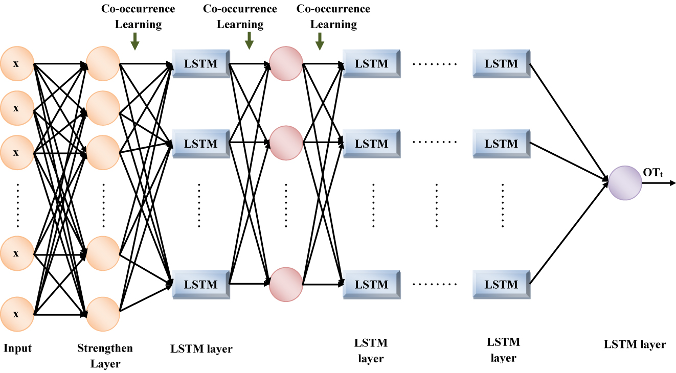
Structure for SGD-DLSTM network.
Input layer: This is to make a decision on what new information was going to accumulate in the cell state. It has ‘2’ parts in it.
A sigmoid layer termed the input gate layer, which decides the values to be updated. The input layer is expressed as,
where, the input layer’s outcome is specified as P t , the activation function is signified as δ(⋅), the input feature values are notated as x i , the weight matrix for the input values is symbolized as α i , the previous hidden layer is exhibited as I t−1, the hidden layer’s weight value is depicted as β i , and the input layer’s bias value is represented as b i .
A ‘tanh layer’ generates a vector of new contender values, which could be appended to the state. The tanh aids in regulating the values flowing via the network. In the range −1 to 1, any real values are taken by the layer. The output value will be closer to 1.0 when the input is larger (more positive), while the output will be closer to −1.0 when the input is smaller (more negative). Next, these two parts are amalgamated to update the state. The tanh expression is computed as,
where, the new cell state is defined as L t , the weight values for input layer and a hidden layer of tanh function are proffered as α l and β l , and the bias value for the new cell state is illustrated as b l .
Strengthen layer: Here, to abate the execution time, the strength betwixt the input layer’s parameters is measured. The useful values are stored only in the subsequent layer by utilizing this layer so that the data can be analysed or reported on. By wielding the covariance computation, the strength is computed as,
Here, the strengthen layer’s outcome is specified as SS
t
, the parameter for the value is signified as ψ
i
, and the parameter for another value is denoted as λ
i
, the mean of ψ is represented as
Forget layer: How much of the prior data will be forgotten and how much of the prior data will be utilized in the further steps will be decided by the forget gate. The details to be eliminated as of the block are detected in this layer. It is decided by a sigmoid function. The sigmoid function exists betwixt (0, 1), this is the reason for utilizing it. Specifically, it is wielded for models for predicting the probability as an output. The sigmoid function is used in the forget gate as the probability of which information needs attention and which can be ignored exists betwixt the range of 0 and 1. For every single number in the cell state L t−1, it looks at the preceding state (L t−1) and the content input (e i ); subsequently, it generates a number betwixt 0 and 1.
where, the forget gate output is denoted as G t , the weight values for the forget gate’s input layer and hidden layer are specified as α g and β g , and the bias value for the forget gate is represented as b g . Now the old cell state G t−1 is updated into the new cell state. The previous steps already decided what to do next. First – The old state multiplies by forgetting the things that were decided to forget earlier. Second – added to the cell state. This is the new candidate value, which is scaled by what proportion is decided to update every state value. The updation is specified as,
The output stage is the final stage. This output is supported by the cell state; however, it will be a filtered version. First, run a sigmoid layer. This layer decides what part of the cell state will be the output.
Output layer: To estimate the output, the block’s input along with memory is utilized. The sigmoid function decides whether to permit 0 or one values. Similarly, the tanh function decides which values should be passed via 0, 1. The weight assigned to the values provided by the tanh function; moreover, determines their significance on a scale of −1 to one and multiplies it with the sigmoid output.
where, the forget gate output is denoted as G t , the weight value for the forget gate’s input values and hidden layer are indicated as α o and β o , and the bias value for the output layer is represented as b o . The Gaussian distribution function is utilized to compute the weight value in all the layers. The Gaussian distribution function is used to compute the weight value in all layers for preventing the layer activation outputs as of exploding or vanishing during a forward pass via a network. It is expressed as,
Here, the Gaussian distribution function is exhibited DI, and the previous layer’s size is depicted as tt.
Deviation analysis
The predicted outcome is assessed following the SPG forecast. This identifies the deviation presented betwixt the predicted outcomes with the original output. In this, for the deviation analysis, the historical data being collected is utilized. Here, MSE, MAE, and RMSE are computed. The predicted value’s absolute distance as of the actual value OT A is evaluated by MAE. The MAE is specified as,
where, the total number of values is indicated as nn. The average of the squared difference betwixt the original and predicted values is termed MSE. The residuals’ variance is measured. The MSE is expressed as,
The errors’ standard deviation that transpired when a prediction is made on a dataset is mentioned as RMSE, which is similar to MSE; however, the root of the value is considered whilst estimating the model’s accuracy.
The forecast’s deviation level is analysed with the aid of all these measures.
Result and discussion
The proposed SPG forecasting model’s performance is assessed in this section. The proposed work is executed in MATLAB. To evaluate the SPG forecasting, the openly accessible dataset was utilized.
Performance analysis
DLSTM, LSTM, RNN, and ANN are the prevailing methodologies with which the proposed methodology is experientially analysed regarding the accuracy, precision, recall, F-Measure, MSE, MAE along with RMSE. Similarly, the proposed IESGO is analogized with the conventional Shell Game Optimizer (SGO), Chaos Game Optimizer (CGO), Soccer Game Optimizer (SGO), and PSO algorithms concerning the fitness versus iteration analysis.
The values attained by the proposed SGD-DLSTM algorithm and existing DLSTM, LSTM, RNN, and ANN algorithms during experimental evaluation are represented in Table 1. As of T, it is established that regarding the accuracy, precision, recall, f-measure, MSE, MAE, and RMSE, better performance was achieved by the proposed SGD-DLSTM algorithm than the prevailing methodologies. Here, the worst performance was shown by the ANN algorithm. This is because ANN is not efficient to recognize the behaviour of nonlinear or dynamic time series, which have moving average terms and hence low forecasting capability. This results in the significance of formulating the model with or without hybrid methodologies. Thus, for the SPG forecasting model, the ANN is not appropriate. Thus, for the SPG forecasting model, the ANN is not appropriate. Consequently, the SGD-DLSTM, which obtains accurate SP output prediction, was utilized by the proposed model.
Demonstrates the performance analysis of the proposed SGD-DLSTM in comparison with the existing algorithm.
| Performance metrics | Proposed SGD-DLSTM | DLSTM | LSTM | RNN | ANN |
|---|---|---|---|---|---|
| Accuracy | 97.25 | 91.42 | 84 | 81.65 | 77.98 |
| Precision | 97.21 | 90.65 | 85.31 | 82.5 | 78.94 |
| Recall | 96 | 92 | 88 | 83.6 | 79.45 |
| F-Measure | 96.6 | 91.32 | 86.63 | 83.04 | 79.19 |
| MSE | 106 | 142 | 165 | 173 | 186 |
| MAE | 7.2 | 8.4 | 8.8 | 9.6 | 10.4 |
| RMSE | 53 | 71.3 | 78 | 93 | 109 |
The accuracy values attained by the proposed system are analogized with the traditional DLSTM, LSTM, RNN, and ANN algorithms in Figure 3. Accuracy proffers how often the presented model predicts the correct output. The graphical representation demonstrates that when analogized with the accuracy values attained by the prevailing DLSTM (91.42%), LSTM (84%), RNN (81.65%), and ANN (77.98%) models, the proposed one attained a higher accuracy of 97.25%.

Accuracy analysis.
In Figure 4, regarding precision, the proposed methodology is analogized with the prevailing methodologies. From the evaluation, it is established that the precision value of 97.21% attained by the proposed model was higher than the ANN by 23.14%; similarly, it is higher than the DLSTM by 7.23%. Therefore, a better performance was achieved by the proposed model than the prevailing DLSTM, LSTM, RNN, and ANN algorithms.

Precision metric analysis for proposed SGD-DLSTM.
The proposed model is compared with the prevailing methodologies in terms of recall in Figure 5. The number of positive outputs computed correctly by the system is proffered as recall. The recall value attained by the proposed model was higher than the ANN and DLSTM algorithms by 20.8% and 4.3%, respectively. Thus, it is evident that the proposed model is highly effectual than the conventional DLSTM, LSTM, RNN, and ANN algorithms.

Analysis of proposed SGD-DLSTM in terms of recall.
Figure 6 exhibits that the f-measure attained by the proposed methodology was 96.6%, which is higher than that obtained by the DLSTM (91.32%) and LSTM (86.63%). Here, the least value of (79.19%) was attained by the ANN; thus, resulting in poor performance. Thus, the best performance was shown by the proposed system when forecasting SPG.

F-measure analysis.
In terms of MSE, the proposed system was analogized with the traditional models in Figure 7. The measure of the average of the squares of the errors is termed MSE. A lower MSE should be produced by a better forecasting model to show better performance. Here, a lower MSE of 106 was attained by the proposed model whereas the prevailing DLSTM, LSTM, RNN, and, ANN methodologies obtained an MSE of 142, 165, 173, and 186, respectively.

Mean square error analysis.
In Figure 8, the proposed model was compared with the prevailing methodologies in terms of MAE. The absolute value of the difference betwixt an observed value of a quantity and the true value is referred to as MAE. The proposed model obtained a lower MAE of 7.2, which is lower than the ANN and DLSTM algorithms by 3.2 and 1.2 errors. Thus, the proposed system’s performance is proved.

Mean absolute error analysis.
The square root of the mean of the square of all the errors is mentioned as RMSE. The RMSE value should be low for better accurate prediction. Figure 9 exhibits that the proposed model attained a lower error value of 53 whereas the prevailing DLSTM, LSTM, RNN, and ANN models attained higher values of 71.3, 78, 93, and 109, in that order. Therefore, it is confirmed that for SPG forecasting, a better performance was achieved by the proposed methodology.

Root mean square error analysis.
In Table 2, regarding fitness versus iteration, the proposed IESGO model is analogized with the prevailing SGO, CGO, SGO, and PSO algorithms. In this, the PSO depicts the worst fitness value. For every iteration, the best fitness values are attained by the proposed system. For 20 iterations, the fitness value attained by the proposed model was 89, which is higher than the fitness values of 74.9, 78.2, 82.6, and 84 attained by the conventional PSO, Soccer Game Optimizer, CGO, and SGO methodologies, respectively. Figure 10 shows the graphical representation of the Fitness versus iteration analysis of the proposed as well as the prevailing methodologies.
Fitness versus iteration analysis.
| Iterations | Proposed IESGO | SGO | CGO | SGO | PSO |
|---|---|---|---|---|---|
| 20 | 89 | 84 | 82.6 | 78.2 | 74.9 |
| 40 | 92.65 | 85.6 | 83.9 | 82.1 | 79 |
| 60 | 95.86 | 87 | 85 | 84.65 | 82.4 |
| 80 | 96 | 91.6 | 89.3 | 87 | 83.5 |
| 100 | 97.2 | 92 | 91 | 88.6 | 85.3 |

Fitness analysis for the proposed IESGO algorithm in comparison with prevailing SGO, CGO, SGO, and PSO algorithms.
Conclusions
In the developing field of Renewable Energy Sources (RESs), to conduct different research works, solar radiation intensity prediction is highly essential. Here, an effectual SGD-DLSTM-centric SPG forecasting system was proposed. IESGO, SGD-DLSTM, and deviation analysis were primarily utilized for designing the proposed model. The SGD-DLSTM preferred for this work offers the benefits of better accuracy, greater generalization performance, along with the immense speed of learning since the weights of DLSTM are computed using the Gaussian distribution function rather than fixed randomly and the strength value regarding the strength of the initialized parameters is maintained using the strengthen layer. Thus, for predicting the SPG, the SGD-DLSTM is wielded for enhancing the DLSTM’s efficacy. By utilizing an openly accessible dataset, the proposed model’s performance was assessed. In performance analysis, regarding the accuracy, precision, recall, F-measure, MAE, MSE, and RMSE, the proposed model’s performance was evaluated with the prevailing DLSTM, LSTM, RNN, and ANN methodologies. A better outcome was obtained by the proposed system than the prevailing methodologies. When compared with the prevailing methodologies, the proposed one attained a better accuracy of 97.25%. Moreover, in terms of fitness versus iteration analysis, the proposed IESGO’s performance was analogized with the prevailing SGO, CGO, SGO, and PSO algorithms. In this also, the proposed model attained a better fitness value. Thus, it is evident that better performance was achieved by the proposed model-centric SPG forecasting. In the future, to enhance SPG forecasting, the proposed framework can be advanced by subsuming additional features with enhanced methodologies.
Abbreviations
- SPG
-
Solar Power generation
- SP
-
Solar Power
- ARIMA
-
Auto-Regressive Integrated Moving Average
- MV
-
Missing Value
- ML
-
Machine Learning
- SVMR
-
Support Vector Machine Regression
- MAE
-
Mean Absolute Error
- RMSE
-
Root Means Square Error
- MSE
-
Means Square Error
- ANN
-
Artificial Neural Networks
- RF
-
Random Forest
- SGD-DLSTM
-
Strengthen Gaussian Distribution-centric Deep Long Short Term Memory
- IESGO
-
Intensive Exploitation-centric Shell Game Optimizer
- DNI
-
Direct Normal Irradiance
- GHI
-
Global Horizontal Irradiance
- DHI
-
Diffuse Horizontal Irradiance
- MSL
-
Mean Sea Level
Acknowledgement
We thank the anonymous referees for their useful suggestions.
-
Author contributions: All authors contributed to the study conception and design. Material preparation, data collection and analysis were performed by *1Surender Rangaraju, 2Dr. Amiya Bhaumik, 3Dr. Phu Le Vo. The first draft of the manuscript was written by *1Surender Rangaraj and all authors commented on previous versions of the manuscript. All authors read and approved the final manuscript.
-
Research funding: This work has no funding resource.
-
Conflict of interest statement: The authors declare no conflicts of interest regarding this article.
-
Ethical approval: This article does not contain any studies with human participants or animals performed by any of the authors.
-
Consent of publication: Not applicable.
-
Availability of data and materials: Data sharing is not applicable to this article as no datasets were generated or analysed during the current study.
References
Awan, S. M., Z. A. Khan, and M. Aslam. 2018. “Solar Generation Forecasting by Recurrent Neural Networks Optimized by Levenberg-Marquardt Algorithm.” In 44th Annual Conference of the IEEE Industrial Electronics Society, 21–23 October 2018, Washington, DC, USA.10.1109/IECON.2018.8591799Search in Google Scholar
Amarasinghe, P. A. G. M., and S. K. Abeygunawardane. 2018. “Application of Machine Learning Algorithms for Solar Power Forecasting in Sri Lanka.” In 2nd International Conference on Electrical Engineering, 28 September 2018, Colombo, Sri Lanka.10.1109/EECon.2018.8541017Search in Google Scholar
Arora, I., J. Gambhir, and T. Kaur. 2020. “Data Normalisation-Based Solar Irradiance Forecasting Using Artificial Neural Networks.” Arabian Journal for Science and Engineering 46 (2): 1333–43, https://doi.org/10.1007/s13369-020-05140-y.Search in Google Scholar
Alaraj, M., A. Kumar, I. Alsaidan, M. Rizwan, and M. Jamil. 2021. “Energy Production Forecasting From Solar Photovoltaic Plants Based On Meteorological Parameters for Qassim Region, Saudi Arabia.” IEEE Access 9: 83241–51, https://doi.org/10.1109/access.2021.3087345.Search in Google Scholar
Aslam, M., S.-J. Lee, and S.-H. Khang. 2021. “Two-Stage Attention Over LSTM with Bayesian Optimization for Day-Ahead Solar Power Forecasting.” IEEE Access 9: 107387–98, https://doi.org/10.1109/access.2021.3100105.Search in Google Scholar
Abdel-Nasser, M., and K. Mahmoud. 2017. “Accurate Photovoltaic Power Forecasting Models Using Deep LSTM-RNN.” Neural Computation & Application 31 (7): 2727–40, https://doi.org/10.1007/s00521-017-3225-z.Search in Google Scholar
Chen, K., Z. He, K. Chen, and J. H. J. He. 2017. “Solar Energy Forecasting With Numerical Weather Predictions on a Grid and Convolutional Networks.” In Conference on Energy Internet and Energy System Integration, IEEE, 26–28 November 2017, Beijing, China.10.1109/EI2.2017.8245549Search in Google Scholar
Chai, S., X. Zhao, Y. Jia, and W. K. Wong. 2020. “A Robust Spatiotemporal Forecasting Framework for Photovoltaic Generation.” IEEE Transactions on Smart Grid 11 (6): 5370–82, https://doi.org/10.1109/tsg.2020.3006085.Search in Google Scholar
Cheng, L., H. Zang, T. Ding, Z. Wei, and G. Sun. 2021. “Multi-Meteorological Factor Based Graph Modeling for Photovoltaic Power Forecasting.” IEEE Transactions on Sustainable Energy 12 (3): 1593–603, https://doi.org/10.1109/tste.2021.3057521.Search in Google Scholar
Fan, T., T. Sun, L. Hu, X. Xie, and Z. Na. 2017. “Spatial Temporal Genetic Based Attention Networks for Short Term Photovoltaic Power Forecasting.” IEEE Access 9: 138762–74, https://doi.org/10.1109/access.2021.3108453.Search in Google Scholar
Huang, C.-J., and P.-H. Kuo. 2019. “Multiple-Input Deep Convolutional Neural Network Model for Short-Term Photovoltaic Power Forecasting.” IEEE Access 7: 74822–34, https://doi.org/10.1109/access.2019.2921238.Search in Google Scholar
Keerthisinghe, C., E. Mickelson, D. S. Kirschen, N. Shih, and S. Gibson. 2020. “Improved PV Forecasts for Capacity Firming.” IEEE Access 4: 1–10, https://doi.org/10.1109/access.2020.3016956.Search in Google Scholar
Kim, H., and D. Lee. 2021. “Probabilistic Solar Power Forecasting Based on Bivariate Conditional Solar Irradiation Distributions.” IEEE Transactions on Sustainable Energy 12 (4): 2031–41, https://doi.org/10.1109/tste.2021.3077001.Search in Google Scholar
Liu, C.-H., J.-C. Gu, and M.-T. Yang. 2021. “A Simplified LSTM Neural Networks for One Day-Ahead Solar Power Forecasting.” IEEE Access 9: 17174–95, https://doi.org/10.1109/access.2021.3053638.Search in Google Scholar
Lee, W., K. Kim, J. Park, J. Kim, and Y. Kim. 2018. “Forecasting Solar Power Using Long-Short Term Memory and Convolutional Neural Networks.” IEEE Access 6: 73068–80, https://doi.org/10.1109/access.2018.2883330.Search in Google Scholar
Li, Q., Y. Xu, B. Chew, H. Ding, and G. Zhao. 2022. “An Integrated Missing-Data Tolerant Model for Probabilistic PV Power Generation Forecasting.” IEEE Transactions on Power Systems 37 (6): 4447–59. https://doi.org/10.1109/TPWRS.2022.3146982.Search in Google Scholar
Munir, M. A., A. Khattak, K. Imran, A. Ulasyar, and A. Khan. 2019. “Solar PV Generation Forecast Model Based on the Most Effective Weather Parameters.” In 1st International Conference on Electrical, Communication and Computer Engineering, 24–25 July 2019, Swat, Pakistan.10.1109/ICECCE47252.2019.8940664Search in Google Scholar
Mukherjee, D., S. Chakraborty, P. K. Guchhait, and J. Bhunia. 2020. “Machine Learning Based Solar Power Generation Forecasting With and Without MPPT Controller.” In International Conference for Convergence in Engineering, 1st International Conference for Convergence in Engineering, IEEE, 5–6 September 2020, Kolkata, India.10.1109/ICCE50343.2020.9290685Search in Google Scholar
Majumder, I., M. K. Behera, and N. Nayak. 2017. “Solar Power Forecasting Using a Hybrid EMD-ELM Method.” In International Conference on Circuits Power and Computing Technologies, IEEE, 20–21 April 2017, Kollam, India.10.1109/ICCPCT.2017.8074179Search in Google Scholar
Sayenko, Y., T. Baranenko and V. Liubartsev. 2020. “Forecasting of Electricity Generation by Solar Panels Using Neural Networks with Incomplete Initial Data.” In 4th International Conference on Intelligent Energy and Power Systems, IEEE, 7–11 September 2020, Istanbul, Turkey.10.1109/IEPS51250.2020.9263085Search in Google Scholar
Serttas, F., F. O. Hocaoglu, and E. Akarslan. 2018. “Short Term Solar Power Generation Forecasting a Novel Approach.” In International Conference on Photovoltaic Science and Technologies, IEEE, 4–6 July 2018, Ankara, Turkey.10.1109/PVCon.2018.8523919Search in Google Scholar
Semero, Y. K., J. Zhang, and D. Zheng. 2018. “PV Power Forecasting Using an Integrated GA-PSO-ANFIS Approach and Gaussian Process Regression Based Feature Selection Strategy.” CSEE Journal of Power and Energy Systems 4 (2): 210–8, https://doi.org/10.17775/cseejpes.2016.01920.Search in Google Scholar
Sheng, H., J. Xiao, Y. Cheng, Q. Ni, and S. Wang. 2016. “Short Term Solar Power Forecasting Based on Weighted Gaussian Process Regression.” IEEE Transactions on Industrial Electronics 65 (1): 300–8, https://doi.org/10.1109/tie.2017.2714127.Search in Google Scholar
Sanjari, M. J., and H. B. Gooi. 2016. “Probabilistic Forecast of PV Power Generation Based on Higher Order Markov Chain.” IEEE Transactions on Power Systems 32 (4): 2942–52, https://doi.org/10.1109/tpwrs.2016.2616902.Search in Google Scholar
Tosun, N., E. Sert, E. Ayaz, E. Yılmaz, and M. Gol. 2020. “Solar Power Generation Analysis and Forecasting Real-World Data Using LSTM and Autoregressive CNN.” In International Conference on Smart Energy Systems and Technologies, IEEE, 7–9 September 2020, Istanbul, Turkey.10.1109/SEST48500.2020.9203124Search in Google Scholar
Tu, C. S., W. C. Tsai, C. M. Hong, W. M. Lin. 2022. “Short-Term Solar Power Forecasting via General Regression Neural Network with Grey Wolf Optimization.” Energies 15 (18): 1–20. https://doi.org/10.3390/en15186624.Search in Google Scholar
Wai, R. J., and P. X. Lai. 2022. “Design of Intelligent Solar PV Power Generation Forecasting Mechanism Combined with Weather Information under Lack of Real-Time Power Generation Data.” Energies 15 (10): 1–30. https://doi.org/10.3390/en15103838.Search in Google Scholar
Yu, Y., J. Cao, and J. Zhu. 2019. “An LSTM Short-Term Solar Irradiance Forecasting Under Complicated Weather Conditions.” IEEE Access 7: 145651–66, https://doi.org/10.1109/access.2019.2946057.Search in Google Scholar
© 2023 Walter de Gruyter GmbH, Berlin/Boston
Articles in the same Issue
- Frontmatter
- Research Articles
- An improved intermittent power supply technique for electrostatic precipitators
- PZT and PVDF piezoelectric transducers’ design implications on their efficiency and energy harvesting potential
- Hybrid optimization for optimal positioning and sizing of distributed generators in unbalanced distribution networks
- Implementation of cascaded H-bridge DC-link inverter for marine electric propulsion drives
- Design of control system for solar power generation based on an improved bat algorithm for an island operation
- Review
- Hybrid renewable energy resources accuracy, techniques adopted, and the future scope abetted by the patent landscape – a conspicuous review
- Research Articles
- Modelling and analysis of green hydrogen production by solar energy
- An economic and technological analysis of hybrid photovoltaic/wind turbine/battery renewable energy system with the highest self-sustainability
- Experimental investigation of Segregated Dry Municipal Solid Waste (SDMSW) and biomass blends in the gasification process
- Energy harvesting for mobile agents supporting wireless sensor networks
- Innovative high-speed method for detecting hotspots in high-density solar panels by machine vision
- Design, simulation and performance analysis of photovoltaic solar water pumping system
- “Design and development of magnetic field harvester to power wireless sensors in smart Grid”
- Modelling of a piezoelectric beam with a full-bridge rectifier under arbitrary excitation: experimental validation
- Multi capacitor modeling for triboelectric nanogenerators with multiple effective parameters
- Sizing electrolyzer capacity in conjunction with an off-grid photovoltaic system for the highest hydrogen production
- A novel SGD-DLSTM-based efficient model for solar power generation forecasting system
- A numerical study of water based nanofluids in shell and tube heat exchanger
- Design of an efficient MPPT optimization model via accurate shadow detection for solar photovoltaic
- Power flow control and power oscillation damping in a 2-machine system using SSSC during faults