Reliability and sensitivity assessment of laminated composite plates with high-dimensional uncertainty variables using active learning-based ensemble metamodels
-
Najib Zemed
 ,
Kaoutar Mouzoun
,
Kaoutar Mouzoun

Abstract
Laminated composite materials play a crucial role in various engineering applications due to their exceptional mechanical properties. This article explores the analysis of reliability and the local sensitivity of failure probability associated with laminated composite materials. It delves into the impact of uncertainties on the performance of these materials and presents an active learning-based reliability methodology. This methodology combines Monte Carlo simulation with a metamodel derived from the combination of three metamodels: artificial neural networks, support vector regression, and Kriging. The article illustrates this methodology through two practical applications on laminated composite plates and compares its performance with other reliability methods. This approach offers valuable insights to enhance the analysis of reliability, strengthen the design process, and facilitate decision-making while fully considering uncertainties related to material properties.
1 Introduction
Laminated composite plates find extensive applications across various sectors, including aerospace, automotive, marine engineering, civil engineering, and renewable energy, due to their outstanding performance and lightweight properties. Their ability to reduce structural weight while preserving strength in comparison to conventional metallic materials is a key driver for their widespread use. Moreover, laminated composites demonstrate superior resistance to both fatigue and corrosion when compared to metals, making them well-suited for enduring use in demanding environments.
To investigate the behavior of composite materials, various modeling theories are employed. Among these, the classical Love–Kirchhoff theory, the oldest, neglects the effects of transverse deformation to predict the behavior of thin plates [1,2]. Subsequently, the first-order shear deformation theory (FSDT) was developed [3], accounting for variations in transverse shear throughout the plate thickness. Furthermore, higher-order shear deformation theories [4,5] were formulated, utilizing increased dependence on the thickness coordinate to describe displacement fields in n-planes. Moreover, research efforts have been made to enhance the modeling of laminate behavior. For instance, Tornabene et al. [6] devised an innovative layer-wise approach employing the generalized differential quadrature (GDQ) method for dynamic analysis of anisotropic shells. They demonstrated the accuracy of their method through numerical examples, aligning with classical 3D finite element predictions in terms of frequencies and mode shapes. In addition, in another study, Tornabene et al. also proposed [7] an equivalent single-layer formulation for linear static analysis of shell structures. They derived fundamental relations from the stationary configuration of total potential energy and addressed them numerically using GDQ. To illustrate their method, they presented several examples demonstrating its effectiveness. Furthermore, Brischetto [8] analyzed the effects of hygrothermal loading on the bending behavior of multilayered composite plates. Using refined two-dimensional models within the framework of Carrera’s unified formulation. Also, Civalek [9] proposed a method of discrete singular convolution to obtain frequencies and buckling loads of composite plates. By utilizing geometric transformation, he then compared the obtained results with those of other numerical methods. However, conducting reliability and sensitivity analyses on these plates under uncertain conditions can be exceptionally challenging, especially when dealing with numerous high-dimensional uncertainty variables. Ensuring the structural integrity and performance of these materials necessitates a meticulous task reliability and sensitivity assessment of laminated composite plates within a high-dimensional uncertainty framework.
The reliability of composite materials fundamentally relies on the use of a limit state function (LSF). This function plays a crucial role by establishing a relationship between the state of the structure and the applied loads. Reliability analysis is typically performed using two main approaches: simulation methods and moment methods. Moment methods are employed to estimate a reliability index, often defined as the distance from the origin to the most probable failure point (MPFP). This index is calculated using algorithms such as the first-order reliability method (FORM) or the second-order reliability method (SORM) [10,11], which rely on linear and nonlinear approximations based on Taylor series expansion of the LSF around the MPFP to estimate the reliability index. While these techniques are fast and efficient, they may lack precision for highly nonlinear problems. To overcome this limitation, Monte Carlo simulations (MCS) have become the preferred and widely used method in various fields [12]. MCS involves generating random samples from probability distributions to model uncertain parameters, followed by performing repeated simulations to estimate the reliability of a system or process. Although this method is highly effective, it can be costly when the probability of failure is very low. To address this issue, several specialized sampling techniques have been developed based on MCS, such as importance sampling (IS) [13–17], subset simulation [18,19], directional simulation [20,21], and line sampling [22,23]. While these approaches require fewer simulations than the MCS, they can still be computationally intensive, especially for complex models that demand significant evaluation time.
For this reason, since the 1990s, several simulation techniques based on metamodels rather than the original model have been developed to reduce the number of necessary evaluations of the LSF. The goal of these techniques is to create a substitute model Y(X) that provides an explicit function to approximate the original performance function. This substitute model is then used in place of the original function in reliability methods. Among these metamodels, there are response surface methods (RSMs) [24,25,26,27], artificial neural networks (ANNs) [28,29,30], radial basis functions [31,32,33], Kriging (also known as Gaussian process) [34,35], support vector machine (SVM), and support vector regression (SVR) [36,37].
Over the past few decades, extensive research has been conducted on the failure and sensitivity of composite materials. For example, Huh [26] employed the stochastic finite element method (SFEM) to assess the reliability of angled plies, comparing results with other reliability methods such as the β-method. The LSF used in this context was based on the Tsai-Wu, Hoffman, and Tsai-Hill criteria. Similarly, Onkar et al. [38] utilized SFEM for reliability analysis, employing the Tsai-Wu and Hoffman criteria as failure criteria for orthotropic plates with random material properties and random loads. Furthermore, recent research on composite reliability has frequently employed metamodels to reduce computational costs. For instance, Lopes et al. [39] employed an ANN to replace the LSF based on the Tsai-Wu failure criterion, demonstrating significant computational efficiency. Dey et al. [40] focused on quantifying thermal uncertainty in the frequency responses of laminated composite plates, using a surrogate model called high-dimensional model representation to propagate thermal, ply-level, and material uncertainties in frequency responses. Chen and Jia [41] investigated interlaminar stress analysis and LSF approximation methods for assessing the reliability of composite structures, discussing the use of surrogate methods such as SVM, RSM, and ANN to approximate the true implicit LSF. Momeni Badeleh et al. [42] have introduced an advanced mesh-free finite volume approach, utilizing it to actively manage the vibrations of a temperature-dependent piezoelectric laminated composite plate based on the principles of first-order shear deformation. The findings indicated a reduction in the reliability of the composite plate with rising temperatures. Martinez et al. [43] conducted a reliability analysis on a smart laminated composite plate comprising a graphite/epoxy cross-ply substrate with a piezoelectric fiber-reinforced composite actuator layer under static electrical and mechanical loads. In their study, they developed a finite element (FE) model in COMSOL Multiphysics, coupled with an ANN and integrated with MCS as well as first- and second-order reliability methods (FORM/SORM). Haeri and Fadaee [44] proposed an efficient and accurate reliability analysis approach for laminated composites called AKM-MCS, employing an advanced Kriging model to approximate the mechanical structure and applying the Tsai-Wu criterion to define LSF. This approach demonstrates high computational efficiency and accuracy. Mathew et al. [45] introduced an innovative approach that combines ANN with the SORM and IS to accurately estimate failure probabilities and sensitivities of variable stiffness composite laminate plates while considering multiple sources of uncertainty. The results demonstrate a high level of accuracy in reliability estimates and sensitivity studies. Finally, Zhou et al. [46] proposed an adaptive Kriging-based approach for the reliability and sensitivity analysis of composite structures with uncertainties, using Kriging to approximate the structural response. This method is applied to composite beams, plates, and random structures, yielding accurate results and efficient reliability evaluation.
Furthermore, to ensure the reliability of composites, it is essential to investigate the contributions of uncertain variables to the behavior of the composite material. This allows for a more precise adjustment of the parameters that have the most significant impact on the probability of failure, a process commonly achieved through the theory of failure probability sensitivity analysis. There are two main types of sensitivity analysis [47]: local reliability sensitivity analysis and global reliability sensitivity analysis. Local reliability sensitivity analysis focuses on quantifying the local effects of distribution parameters of random input variables on the failure probability [48]. Its objective is to rank these distribution parameters based on their impact on the failure probability. On the other hand, global reliability sensitivity analysis assesses the contributions of uncertainties present in the input variables to the failure probability [49]. It ranks these sources of uncertainty based on their impact on the failure probability.
This article introduces an approach to analyze the reliability and local sensitivity of the failure probability of composite materials using an LSF that incorporates the criteria of maximum stress, Tsai-Hill, and Tsai-Wu. The reliability methodology relies on an active learning method that combines MCS with a metamodel resulting from a weighted combination of three metamodels: ANN, SVR, and Kriging. The weighting coefficients for these three metamodels are determined through a heuristic method (Goel et al.). This approach provides valuable insights into the behavior and performance of laminated composites, contributing to the enhancement of design and decision-making processes while considering uncertainties related to material properties. Two applications on flat composite laminates were used to test this method and to demonstrate its effectiveness.
2 Failure theory
Failure theories play a central role in assessing the robustness of structures. In the context of composite materials, this fundamental discipline aims to understand the mechanisms and conditions leading to the rupture or degradation of these materials. It relies on the analysis of stresses, loads, and the study of interactions within the composite structure, while seeking to anticipate potential failure modes. Several failure criteria have been developed to assess the strength of composites in various loading scenarios. These criteria are generally categorized into two main groups:
Simple limit failure theories, such as the maximum stress criterion,
Interaction theories, such as the Tsai-Hill and Tsai-Wu criteria.
2.1 Maximum stress criterion
The maximum stress criterion is one of the primary failure criteria used to assess the strength of composite materials. This criterion is based on the concept that failure occurs when a material exceeds its maximum stress-carrying capacity in one of its directions. In other words, if any of the principal stresses applied to a composite material exceeds its corresponding strength, failure occurs.
To apply this criterion, the principal stresses computed within the structure are compared with the material’s maximum strengths in each direction. Failure happens when one of the following inequalities is not satisfied:
where σ 1 , σ 2, and σ 3 represent the principal components of normal stresses, and σ 4 , σ 5, and σ 6 represent the principal components of shear stress, while X t, Y t, Z t, X c, Y c, and Z c correspond to the ultimate tensile and compressive strengths of the lamina in the 1, 2, and 3 directions, and R, S, and T denote the ultimate shear strengths of the lamina in the 2–3, 1–3, and 1–2 planes, respectively.
For a 2D in-plane stress state (σ 3 = 0, σ 4 = 0, σ 5 = 0), which is often the case for laminates, the maximum stress failure criterion is expressed as follows:
2.2 Tsai-Hill criterion
The Tsai-Hill failure criterion is based on the concept of distortion energy [50]. It is an adaptation of the Von Mises criterion, initially designed for isotropic materials, but it has been specifically tailored for anisotropic materials like composites. This failure criterion assesses the strength of a composite material by considering the intricate interactions between stresses and strains that occur in an anisotropic material.
The failure condition according to the Tsai-Hill criterion is defined as follows:
where the values of X, Y, and Z represent X t, Y t, Z t or X c, Y c, and Z c depending on the sign of σ 1, σ 2, and σ 3.
For a 2D in-plane stress state (σ 3 = 0, σ 4 = 0, σ 5 = 0), the Tsai-Hill failure criterion is expressed as follows:
2.3 Tsai-Wu criterion
The Tsai-Wu criterion is a widely used failure model for assessing the safety of composite materials. It is based on Beltrami’s theory of failure by total strain energy [51]. According to this criterion, a lamina or composite material is considered to fail if the following inequality is not satisfied:
where
For a 2D in-plane stress state (σ 3 = 0, σ 4 = 0, σ 5 = 0), the Tsai-Wu failure criterion is expressed as follows:
3 Reliability and probability of failure sensitivity theory
3.1 Failure probability
The failure probability of structures is defined through the LSF G(x). This probability is defined as the percentage of the region in which the LSF G(x) is less than zero. It is calculated using the following integral:
where
The failure probability can be expressed as follows:
where E represents the expectation function with respect to
The integral in Eq. (8) is complex to solve directly. For this reason, the MCS is employed to estimate this integral. This method involves generating a population, denoted as P, which is then used to simulate the system N times. The number of failure events is counted, and therefore, the probability of failure can be estimated by the following expression:
Furthermore, to obtain a reliable degree of precision for this result, it is necessary to calculate the coefficient of variation (CoV) of
In most cases, a precision level of CoV < 0.05 is commonly employed, as indicated by researchers [52,53].
3.2 Local sensitivity of failure probability
The primary objective of local sensitivity analysis of failure probability is to measure the local impacts of the distribution parameters of input random variables on the failure probability. It has been employed in the context of probability by the researcher [48]. To achieve this, the gradient of the failure probability with respect to these variables is evaluated:
where
Furthermore, to ensure a fair comparison of the sensitivities of all random variables in the studied system, it is necessary to standardize these sensitivities with respect to the probability of failure, making them dimensionless. A normalization method proposed by Wu and Mohanty [54] is expressed as follows:
where
This sensitivity can be estimated using the MCS method:
If the input variables are independent, the joint density can be decomposed into
According to Wu [48], two types of sensitivity can be defined, the first one being sensitivity of the probability of failure with respect to the mean μ, and the second one with respect to the standard deviation σ:
4 Reliability and sensitivity analysis method based on an ensemble of metamodels
The proposed reliability and sensitivity approach is based on an ensemble of metamodels, involving the creation of a set of metamodels designed to simulate the LSF G(X). These metamodels are subsequently utilized to assess the probability of failure and its sensitivity, replacing the LSF itself. This approach is typically characterized by five key features:
The formulation of an LSF specifically adapted to composite laminates based on failure criteria.
The construction of an average and robust metamodel, which combines three distinct metamodels weighted by coefficients.
The use of an active learning method through a proposed learning function enables the intelligent selection of samples to be added to the experimental plan.
The evaluation of a stopping criterion tailored to this approach ensures proper convergence of results towards the exact
The estimation of the probability of failure and the local sensitivity of the probability of failure using MCS, in conjunction with the constructed average metamodel.
The key characteristics of this approach are presented below.
4.1 LSF incorporating failure criteria
In the context of reliability analysis theory, failure is always described using an LSF, denoted as G(X). This function establishes a relationship between the limit state of the structure and various factors, including applied loads, material properties, and other relevant parameters. In this research, to ensure the reliability and safety of composites, and since none of the failure criteria guarantee the most conservative results in all conditions according to Martinez and Bishay [55], it is assumed that failure occurs when one of the three failure criteria is satisfied. To this end, an LSF based on the failure criteria presented in the previous section has been defined as follows:
where X = {x 1 , x 2,…, x n } represents the vector of input random variables, which typically include loads and material properties, and the failure occurs when the LSF has a negative value, G(X) ≤ 0.
4.2 Construction of a metamodel combining three metamodels
To construct a consolidated average metamodel from multiple metamodels, the commonly used method is the metamodel ensemble approach, which has been recently incorporated into structural reliability analysis by researchers [56,57]. This approach involves training multiple metamodels using the same sample points and then combining them to obtain a more accurate prediction than what each individual model could provide separately. The combination of these metamodels is achieved by determining the weights associated with each of them.
In the literature, there are two primary strategies for determining these weights. First, there is global weighting, where the weights w i are constant for each metamodel ŷ i . This includes methods such as weight calculation based on root-mean-square error (RMSE) [58], Bayesian model averaging [59], or determining weights using an optimization problem [42]. Second, there is local weighting, where the weights depend on input values X. An example of this is variance-based local weighting [60].
In this article, the method of weight calculation based on RMSE [58] is employed. This method suggests the calculation of the average metamodel using the following formula:
where Ŷ ens(x) represents the global prediction of the EM at given x, ŷ i represents the output of the ith meta-model at the specific point x, M stands for the total number of surrogates employed in the EM, and w i corresponds to the weight assigned to the ith meta-model.
Moreover, this approach enables the detection of regions where substantial prediction errors may occur by computing the variance
The weights are computed using a heuristic formulation that employs a “leave-one-out” cross-validation strategy to determine the RMSE. The weight calculation is as follows:
where Y (k) represents the real response at a given point x (k), Ŷ (k) represents the predicted response obtained from the ith surrogate model trained using all points of the design of experiments (DoEs) except the pair (x (k), y (k)), and N DoE is the total number of DoE, and α and β are two parameters that need to be defined. In this article, the same parameter values as those used by Goel et al. [58] have been applied, α = 0.05 and β = −1.
4.3 U EM learning function
The accuracy of determining the failure probability largely depends on the precise classification of points near the system’s state limit, where Y(x) = 0. To ensure this precision, Echard et al. [53] implemented the U-learning function, which was developed in the context of the AK-MCS algorithm. This function identifies points that may potentially cross the predicted separator of the metamodel Ŷ(x) = 0 incorrectly.
In this article, an adaptation of this LSF has been introduced. It involves the introduction of a minimum distance between the studied point and the points already present in the design of experiments. This adaptation aims to achieve a balanced distribution of all samples in the space, preventing excessive point concentration in a single area and ensuring a uniform distribution. This learning function is defined as follows.
where Ŷ
ens(x) represents the global prediction of the EM at given x,
4.4 Stopping criterion for the algorithm
The stopping criterion adopted in this method is based on the evolution of the failure probability values over the last five iterations and is proposed as follows:
where i represents the value of the last iteration and
4.5 Calculation of failure probability and its sensitivity
The U EM learning function is computed for all points in the population. The point with the lowest value is then incorporated into the DoE. The best next point, denoted as X*, is then determined by:
At each iterative step, X* is identified and incorporated into the DoE. Subsequently, metamodels are refined using this new DoE, and the failure probability is calculated at each iteration according to the following expression:
Then, the local sensitivity of the failure probability is calculated according to the following expression:
5 Metamodels employed in the proposed method
In this section, the theories of the metamodels used in the ensemble metamodel method are presented, namely, ANN, SVR, and Kriging.
5.1 ANN
ANNs, a subset of machine learning, form the cornerstone of deep learning algorithms. They draw their name and structure from the human brain, aiming to simulate how the human brain processes information. These networks consist of layers of nodes, including an input layer, one or more hidden layers, and an output layer. Each node is interconnected with others and is assigned an associated weight (W i ), as depicted in Figure 1.

ANNs architecture.
Each neuron transforms the input into an output using an activation function, which has the role of introducing a nonlinearity in the output of a neuron, and in this study, we use the sigmoid function as activation function, which is defined as follows:
At the level of each neuron, a weighted set of inputs from the previous layer is summed, and the activation function is applied to this sum as follows:
where,
Considering that the sigmoid function is sensitive in the interval [−1,1], we proceed to normalize all inputs and outputs (targets) as described by Rafiq et al. [61]:
For inputs:
where S is the normalized value of the variable X and X min and X max are the minimum and maximum values of the variables.
For targets:
where
In this study, an ANN was employed, featuring three hidden layers, each comprising 20 nodes. To determine the problem’s weight values, the Levenberg-Marquardt (LM) algorithm implemented in MATLAB was utilized to address the nonlinear least squares problem.
5.2 SVR
SVR is an evolution of the SVM that expands its capabilities. It introduces the concept of an ε-insensitive tube, as illustrated in Figure 2. Within this tube, deviations from the target output are allowed without any penalties, while outside the tube, penalties are applied to deviations. SVR is fundamentally a machine learning algorithm [36] that relies on a loss function L ε called e-insensitive function. This function is designed to handle cases where we are less concerned with small deviations within the ε tube but want to penalize larger deviations outside it, making SVR particularly useful for robust regression tasks. This loss function L ε is defined as follows:

Curve of the SVR approximation function with the slack variables.
5.2.1 Linear case
In the linear case, f(x) is defined as follows:
where
According to Vapnik [36,37], achieving a flat approximation linear function implies maximizing the margin, and this objective can be accomplished by minimizing the Euclidean norm of w, which means
where
This approximation assumes that all inputs exist inside the ε-tube, but this is not always the case, so slack variables ξ i , ξ i * are introduced, and this optimization problem becomes:
where the constant C > 0 plays a crucial role in determining the balance between achieving a flat approximation (small w) and the tolerance level for deviations exceeding ε.
To solve the optimization problem with the linear constraints, the Lagrangian function is used:
where
For optimality, according to the Lagrangian theory, it is necessary for the partial derivatives of L with respect to each variable to vanish.
To solve the Lagrangian optimization in Eq. (38), it is preferable to solve it in its dual formulation, by substituting Eq. (39) into Eq. (42) in Eq. (38), yields the dual formulation, which depends only on α i :
5.2.2 Nonlinear case
For the nonlinear case, a nonlinear projector Φ is used, which has the objective of transforming the starting space to a space of higher dimension than the starting one,
This function K represents the dot product between two projections. In this context, the Lagrangian optimization problem can be expressed as follows:
From Eq. (39), and considering the projection function
To calculate the offset b, the Karush–Kuhn–Tucker condition [62] are utilized, These conditions state that the product between the constraints and the Lagrange multipliers must equal zero at the optimal solution. This implies:
Then, the approximation function is written as:
5.3 Kriging metamodel
The Kriging model, a nonlinear interpolation meta-model developed for Geostatistics by Matheron [63], also known as Gaussian process, is a statistical interpolation method employed to predict or estimate unknown values within a given space by utilizing observations made at various points within that space. This approach is based on establishing a stochastic random field that simulates the behavior of the limit function. Subsequently, the technique known as the best linear unbiased predictor (BLUP) is utilized to optimally estimate the value of this model at a specific point. The Kriging function is written as a realization of a random function as described by [64].
where
Z(x) is a stationary Gaussian process that has an unknown form, zero mean and the following covariance functions between two points of space:
where σ is the variance of the process and
In this type of Kriging, the Gaussian process is stationary, which means that the autocorrelation function R depends only on the difference between the points and on a set of hyperparameters
where i, j = 1,., n, with n representing the number of random variables, and N 0 denoting the number of points in the design of experiments.
The identification of the hyperparameters
where
Then, since maximizing this likelihood is equivalent to minimizing its opposite natural logarithm, the first-order optimality conditions for this likelihood logarithm is used to determine the two estimations of the parameters β and σ 2.
These two equations lead to:
However, the two parameters in Eqs. (55) and (56) depend on the correlation parameter θ, so it is first necessary to obtain it using maximum likelihood estimation:
By expanding the optimization problem of the Eq. (57) and eliminating the constant terms, the likelihood function is reduced to:
After the determination of the parameter θ, the best linear unbiased predictor (BLUP) is used to determine
where
where
To build the Kriging model in this article and to solve the global optimization problem of Eq. (58), which is complex and cannot be solved analytically, an optimization algorithm is developed in MATLAB to solve this problem.
6 Algorithm of the proposed methodology
The methodology developed in this article for reliability analysis and sensitivity to reliability is organized into three main stages. The implementation details of this method are described below and illustrated in Figure 3.

Algorithm of the methodology used for calculating the reliability and sensitivity of composite materials.
6.1 Stage 1: convergence analysis and numerical validation
This stage holds paramount significance within our methodology, aiming to validate the FE model and determine the optimal mesh to use. The first substage involves validating the obtained results by comparing them with analytically calculated results. Subsequently, the second substage aims to determine the optimal mesh size. It is well known that a finer mesh yields more precise results, albeit often at the cost of longer computational time. Therefore, a convergence study becomes necessary, employing various mesh sizes to ascertain the optimal size that provides both adequate accuracy and reasonable computation time.
Moreover, in the absence of precise analytical results, it is conceivable to assess the model’s validation and convergence by comparing it to other established finite element models based on different theories or concepts. Alternatively, running it within a different finite element software is also a viable approach.
6.2 Stage 2: reliability analysis
The objective of this stage is to achieve a precise estimation of failure. It includes the following steps:
Generate the Monte Carlo population S using Latin hypercube sampling (LHS) technique.
Select from S a number N 0 (e.g., N 0 = 12) of points X = {X 1,…,
Build the three metamodels Kriging–ANN–SVR using {X, Y} and determine the metamodel mean
Estimate the failure probability
(61)Evaluate the stopping criterion in Eq. (46). If the condition is met, proceed to the next stage; otherwise, find the best point X* from all points in S to add it to the DoE, by minimizing the learning function U EM. Then calculate the response Y(X*). Next, update the
Calculate the coefficient of variation of
6.3 Stage 3: reliability sensitivity analysis
Once the failure probability calculation algorithm is completed, the sensitivity of the failure probability with respect to a given parameter θ i is estimated using the following expression:
7 Numerical results and discussion
Numerical analysis was conducted on two graphite/epoxy T300/5208 composite plates examined by [65]. The first composite plate is characterized by an antisymmetric angle-ply configuration [−45°, 45°, −45°, 45°], subjected to a uniformly distributed transverse load. The second composite plate adopts a symmetric cross-ply arrangement [0°, 90°, 90°, 0°], and it experiences uniaxial loading on one side only.
Reliability analysis for these two applications was conducted using three different methods to ensure the reliability of the results and facilitate comparisons between these methods. The three methods employed are the MCS method, the proposed method in this article, and the well-known AK-MCS method [53], which serves as a reference for new approaches based on machine learning. It is worth noting that, for the AK-MCS method, we utilized its proposed stopping criterion rather than its original one to ensure a fair and consistent comparison.
Local sensitivity analysis was conducted to assess the sensitivity of failure probability with respect to changes in the mean and standard deviation of input variables. This sensitivity was calculated using the reliability results obtained from the three methods employed to evaluate the laminate’s reliability. A positive sensitivity indicates that when the mean of a variable increases, the probability of failure also increases, while a negative sensitivity suggests the opposite, namely, that an increase in the mean of a variable decreases the probability of failure.
7.1 Techniques and applications utilized
7.1.1 Tools and software
The simulations were conducted using the ANSYS APDL software with the SHELL181 finite element, which provides six degrees of freedom at each node, as illustrated in Figure 4. This software was used to model the laminates. Furthermore, the necessary codes for performing reliability analysis and sensitivity analysis were developed within the MATLAB environment. A coupling between the two software tools was established.

Quadrilateral four-node shell element in ANSYS software (SHELL181).
This element is based on the FSDT, which assumes that the transverse deformation through the thickness is constant and also takes into account the transverse shear displacement. The parameter settings and assumptions used for this element in ANSYS are as follows:
KEYOPT(1) = 0: This parameter is set to include both membrane forces and moments in the calculation of the element stiffness.
KEYOPT(3) = 0: It is set to zero to utilize reduced integration, which reduces computational time while maintaining acceptable accuracy.
KEYOPT(5) = 1: This option selects the standard formulation of the shell under the FSDT theory.
KEYOPT(8) = 3: By setting this parameter to 3, results are computed at the top, bottom, and mid-plane of each layer, allowing us to subsequently assess failure criteria at three points for each layer, aiming to ensure more reliable results.
KEYOPT(9) = 0: No subroutine is used to provide initial thickness, meaning that thickness data is directly defined within the model.
KEYOPT(10) = 0: By default, the normal stress is assumed to be zero.
KEYOPT(11) = 0: The standard orientation axes of the element are used by default.
7.1.2 Transformation of stress to the local coordinate systems of each laminate layer
In the context of evaluating failure criteria, it is imperative to analyze stresses and strains with respect to the material axes specific to each constituent layer of the laminate. However, it is common for the intrinsic axes of the laminate not to align with the principal axes of individual layers. Since the stresses predicted by ANSYS are calculated with respect to the global axes (σ xx , σ yy , σ zz , τ yz , τ xz , τ xy ), a transformation using MATLAB is performed to determine the principal stresses (σ 1 , σ 2 , σ 3 , σ 4 , σ 5 , σ 6) for each laminate. This transformation is carried out using the following matrix:
7.2 Convergence analysis and validation of the FE model
A FE validation study was conducted to confirm the accuracy of the model. Furthermore, a convergence study was carried out by varying the mesh size (2 × 2), (4 × 4), (6 × 6), (8 × 8), and (10 × 10) to determine the optimal mesh, allowing for precise analytical results while minimizing resource utilization and computation time. Precise deflection values for the plates were extracted from the research of Reddy and Pandey [65,66]. The properties of the epoxy graphite material T300/5208 and the applied force for this validation are presented in Table 1.
Applied force and mechanical properties of epoxy graphite material T300/5208
| Parameter | Description | Unit | Value |
|---|---|---|---|
| E 11 | Elastic modulus in the 11 direction | MPa | 132,500 |
| E 22 | Elastic modulus in the 22 direction | MPa | 10,800 |
| v 12 | Poisson’s ratio in the 12 direction | — | 0.24 |
| G 12 | Elastic modulus in the 12 direction | MPa | 5,700 |
| G 13 | Elastic modulus in the 13 direction | MPa | 5,700 |
| G 23 | Elastic modulus in the 23 direction | MPa | 3,400 |
| L | Length of the laminate | m | 0.2286 |
| l | Width of the laminate | m | 0.127 |
| t | Thickness of the laminate | m | 0.000127 |
| X T | Tensile strength of the laminate in the 11 direction | MPa | 1,515 |
| X c | Tensile strength in the 22 and 33 directions | MPa | 1,697 |
| Y T & Z T | Compression strength in the 22 and 33 directions | MPa | 43.8 |
| Y c & Z c | Compression strength in the 22 and 33 directions | MPa | 43.8 |
| R | Shear strength in the 23 direction | MPa | 67.6 |
| S & T | Shear strength in the 13 and 12 directions | MPa | 86.9 |
| P | Applied surface force | MPa | 0.000689476 |
The results, presented in Table 2, indicate that the maximum deflection values obtained from numerical simulations of the plate are nearly equal to the exact solutions. This confirms the validation of the FE-based model. Furthermore, in the analysis of results convergence based on mesh size, the choice was made to use the (8 × 8) mesh for all subsequent steps. This selection is justified by its ability to provide sufficiently accurate results compared to the exact solution while exhibiting minimal differences compared to the next mesh size, which is (10 × 10).
Results of the study on FE model validation and convergence
| Laminate | Solution found by FEM (mm) | Exact solution (mm) [58] | Error (%) | ||||
|---|---|---|---|---|---|---|---|
| Mesh | (2 × 2) | (4 × 4) | (6 × 6) | (8 × 8) | (10 × 10) | — | — |
| [−45°, 45°, −45°, 45°] | 2.6740 | 2.8148 | 2.7713 | 2.7654 | 2.7634 | 2.7609 | 0.0877 |
| [0°, 90°, 90°, 0°] | 5.4153 | 5.8615 | 5.8451 | 5.8364 | 5.8323 | 5.8166 | 0.2699 |
7.3 Example 1: Composite plate under Uniformly distributed transverse load
The first example involves a laminated composite plate consisting of 4 layers with an antisymmetric angular arrangement [−45°, 45°, −45°, 45°] made of graphite/epoxy T300/5208, as depicted in Figure 5. This laminate is simply supported at its edges and subjected to a uniformly distributed load over its surface. Dimensional characteristics such as length, width, and thickness, as well as the properties of the graphite/epoxy material (elasticity modules in different directions, Poisson’s ratio in direction 12, maximum strengths in different directions), and the applied surface force are all considered as random variables in this example. The probability distributions of these variables are presented in Table 3.

Composite plate under uniformly distributed transverse load.
Random variable distribution of the antisymmetric angle-ply [−45°, 45°, −45°, 45°]
| Variable | Description | Unit | Mean value | Standard deviation | Distribution |
|---|---|---|---|---|---|
| E 11 | Elastic modulus in the 11 direction | MPa | 132,500 | 13,250 | Normal |
| E 22 | Elastic modulus in the 22 direction | MPa | 10,800 | 1,080 | Normal |
| v 12 | Poisson’s ratio in the 12 direction | — | 0.24 | 0.024 | Normal |
| G 12 | Elastic modulus in the 12 direction | MPa | 5,700 | 570 | Normal |
| G 13 | Elastic modulus in the 13 direction | MPa | 5,700 | 570 | Normal |
| G 23 | Elastic modulus in the 23 direction | MPa | 3,400 | 340 | Normal |
| L | Length of the laminate | m | 0.2286 | 0.02286 | Normal |
| l | Width of the laminate | m | 0.1270 | 0.002 | Normal |
| t | Thickness of the laminate | m | 0.000127 | 0.0000127 | Normal |
| X T | Tensile strength of the laminate in the 11 direction | MPa | 1,515 | 151.5 | Normal |
| X C | Tensile strength in the 22 & 33 directions | MPa | 1,697 | 169.7 | Normal |
| Y T & Z T | Compression strength in the 22 & 33 directions | MPa | 43.8 | 4.38 | Normal |
| Y C & Z C | Compression strength in the 22 & 33 directions | MPa | 43.8 | 4.38 | Normal |
| R | Shear strength in the 23 direction | MPa | 67.6 | 6.76 | Normal |
| S & T | Shear strength in the 13 & 12 directions | MPa | 86.9 | 8.69 | Normal |
| P | Applied surface force | MPa | 0.0035 | 0.00035 | Gumbel |
7.3.1 Reliability analysis of the composite plate
The reliability results for the laminate are presented in Table 4. The exact probability was computed using the MCS method with 100,000 simulations. It is noteworthy that the proposed method yielded results very close to the exact value, with an estimation error of only 2.27% compared to the MCS method. Furthermore, it is important to highlight that the proposed method required only 102 simulations to achieve this probability, which is significantly fewer than the simulations needed by the AK-MCS method.
Results of reliability analysis for the antisymmetric angle-ply composite [−45°, 45°, −45°, 45°]
| Method | Number of calls |
|
Error (%) |
|---|---|---|---|
| MCS | 100,000 | 0.009131 | — |
| AK-MCS [53] | 12 + 159 = 171 | 0.009596 | 5.09 |
| Proposed method | 12 + 90 = 102 | 0.009339 | 2.27 |
Figure 6 illustrates the evolution curve of the estimated failure probability using the proposed method and the AK-MCS method. It can be observed that the proposed method rapidly converged to the exact solution starting from the 86th iteration, and the algorithm did not require many simulations to meet the stopping criterion, as it reached it after only about 16 additional simulations. In contrast, the AK-MCS method required a much higher number of simulations to meet the same stopping criterion.

Evolution of probability for example 1.
Figure 7 presents the evolution of weighting coefficients associated with the three metamodels used in the proposed method. Overall, it can be observed that the Kriging metamodel dominates in the initial and final segments of the curve, while in the central part of the curve, covering approximately one-third, the SVR metamodel takes precedence at certain points. On the other hand, the ANNs metamodel consistently maintains low weights in comparison to the other two, except in 3 out of the 102 iterations where it outperforms the other two metamodels.

Evolution of weight contribution of metamodels for example 1.
7.3.2 Sensitivity analysis of the composite plate
Figures 8 and 9, respectively, depict the sensitivity of failure probability regarding the mean and standard deviation of variables. It is clearly observed that the thickness t of the laminate layers has a significant impact on the failure probability. Furthermore, given its positive sensitivity to the mean, it can be affirmed that it positively contributes to the increase in the failure probability. Variables such as Young’s moduli E 11 and E 22, as well as the maximum strengths Y T /Z T and Y C /Z C, length L, width l, and force P exhibit almost the same level of impact. Among these, E 22, L, l, and P significantly contribute to the failure probability, while E 11, Y T /Z T, and Y C /Z C have a reducing effect on the failure probability. As for the remaining variables, their impact on the failure probability is negligible.

Sensitivity of failure probability to the mean of variables for example 1.

Sensitivity of failure probability to the standard deviation of variables for example 1.
To enhance reliability and reduce the probability of failure of this composite plate, it is imperative to take appropriate measures. Based on the results of our sensitivity analysis, it is evident that enhancing the robustness of critical variables is essential. Specifically, by prioritizing the optimization of the thickness t of the laminate layers and selecting high-quality composite materials characterized by high Young’s modulus E 11 and optimal maximum strengths (Y T /Z T and Y C /Z C), while ensuring that dimensions (length and width) align with the required specifications, it becomes feasible to significantly diminish the probability of failure. This proactive approach will bolster the overall resilience of the structure and promote a more dependable performance of the composite plate.
7.4 Laminates with hole under in-plane loading
The second example is a laminated composite plate comprising 4 layers, arranged in a symmetric cross-ply configuration [0°, 90°, 90°, 0°], made of graphite/epoxy T300/5208, and featuring a circular hole at the center of the plate. This laminate is clamped on one side and simply supported on the other, while being subjected to a linear tensile load on that side, as illustrated in Figure 10.

Composite laminates with a hole under in-plane loading.
In the context of this example, given the absence of an analytical solution to validate the FE model, the structure was modeled using two types of predefined FEs in the ANSYS software, namely, shell181 and shell281. A comparison of the displacement results for the node located at the center of the edge under a uniformly distributed load revealed consistency between the two approaches.
Regarding meshing, a specific strategy was employed, with an increase in density near the central hole and a decrease in other areas. To assess mesh convergence, various mesh sizes were utilized, gradually decreasing. The optimal mesh size was chosen by observing that the lateral displacement results of the specified node showed no significant improvement for smaller meshes, while maintaining stability for the larger mesh.
In this example, the maximum strengths in different directions are considered constant and are presented in Table 1. The variables in this problem are the length, the width, the thickness of each layer, the radius of the hole, the fiber orientation for each layer, the elastic modulus in different directions, Poisson’s ratio in direction 12, and the applied linear force. The probability distributions of these variables are presented in Table 5.
Random variable distribution of the symmetric cross-ply [0°, 90°, 90°, 0°]
| Variable | Description | Unit | Mean value | Standard deviation | Distribution |
|---|---|---|---|---|---|
| E 11 | Elastic modulus in the 11 direction | MPa | 13,2500 | 13,250 | Normal |
| E 22 | Elastic modulus in the 22 direction | MPa | 10,800 | 1,080 | Normal |
| v 12 | Poisson’s ratio in the 12 direction | — | 0.24 | 0.024 | Normal |
| G 12 | Elastic modulus in the 12 direction | MPa | 5,700 | 570 | Normal |
| G 13 | Elastic modulus in the 13 direction | MPa | 5,700 | 570 | Normal |
| G 23 | Elastic modulus in the 23 direction | MPa | 3,400 | 340 | Normal |
| L | Length of the laminate | m | 0.2286 | 0.02286 | Normal |
| l | Width of the laminate | m | 0.127 | 0.002 | Normal |
| d | Subtracted hole diameter | m | 0.0254 | 0.00254 | Normal |
| t 1 | Thickness of laminate 1 | m | 0.000127 | 0.0000127 | Normal |
| t 2 | Thickness of laminate 2 | m | 0.000127 | 0.0000127 | Normal |
| t 3 | Thickness of laminate 3 | m | 0.000127 | 0.0000127 | Normal |
| t 4 | Thickness of laminate 4 | m | 0.000127 | 0.0000127 | Normal |
| θ 1 | Fiber orientation in laminate 1 | ° | 0 | 5 | Normal |
| θ 2 | Fiber orientation in laminate 2 | ° | 90 | 5 | Normal |
| θ 3 | Fiber orientation in laminate 3 | ° | 90 | 5 | Normal |
| θ 4 | Fiber orientation in laminate 4 | ° | 0 | 5 | Normal |
| N x | Linear force applied | MN/m | 0.045 | 0.0045 | Gumbel |
7.4.1 Reliability analysis of the composite plate
The reliability results for the laminate are presented in Table 6. The exact probability was computed using the MCS method with 50,000 simulations. It is observed in the table that the proposed method yielded an acceptable result with an error of 9.14%, and it achieved this with only 154 simulations. In contrast, the AK-MCS method required a larger number of simulations to produce a result with a greater error than the proposed method.
Results of reliability analysis for the symmetric cross-ply [0°, 90°, 90°, 0°]
| Method | Number of calls |
|
Error (%) |
|---|---|---|---|
| MCS | 50,000 | 0.0339 | — |
| AK-MCS [53] | 12 + 241 = 253 | 0.0396 | 16.81 |
| Proposed method | 12 + 142 = 154 | 0.0308 | 9.14 |
The evolution of failure probability as a function of the number of simulations is presented in Figure 11, illustrating the trajectory of the estimated failure probability using both our proposed method and the AK-MCS method. It is remarkable that our method converged to the exact solution by the 154th iteration, while the AK-MCS method required 253 simulations to reach the same stopping criterion. Therefore, it is encouraging to note that our method required a relatively modest number of simulations, especially considering the large number of random variables involved, totaling 18 variables.

Evolution of probability for example 2.
Figure 12 shows the evolution of the weighting coefficients of the three meta-models used in the proposed method. In this example, the Kriging meta-model does not dominate as much as in the previous example. In fact, it can be observed that the three metamodels almost equally contributed throughout the process. This shows the advantage of this approach, which combines the strengths of each meta-model by assigning them different weights based on their accuracy.

Evolution of weight contribution of metamodels for example 2.
7.4.2 Sensitivity analysis of the composite plate
Figures 13 and 14, respectively, illustrate the sensitivity of failure probability concerning the mean and standard deviation of variables. It is evident that the mechanical properties of the laminates have a negligible impact on the probability of failure. However, regarding the thickness of the laminates, only the thicknesses t 2 and t 3, corresponding to laminates with fibers oriented at 90°, have moderate and negative effects on the probability of failure. Concerning the dimensions of the laminate, the length L of the laminate has no effect, while the width and hole diameter have a significant impact on the probability of failure, with negative and positive effects, respectively.
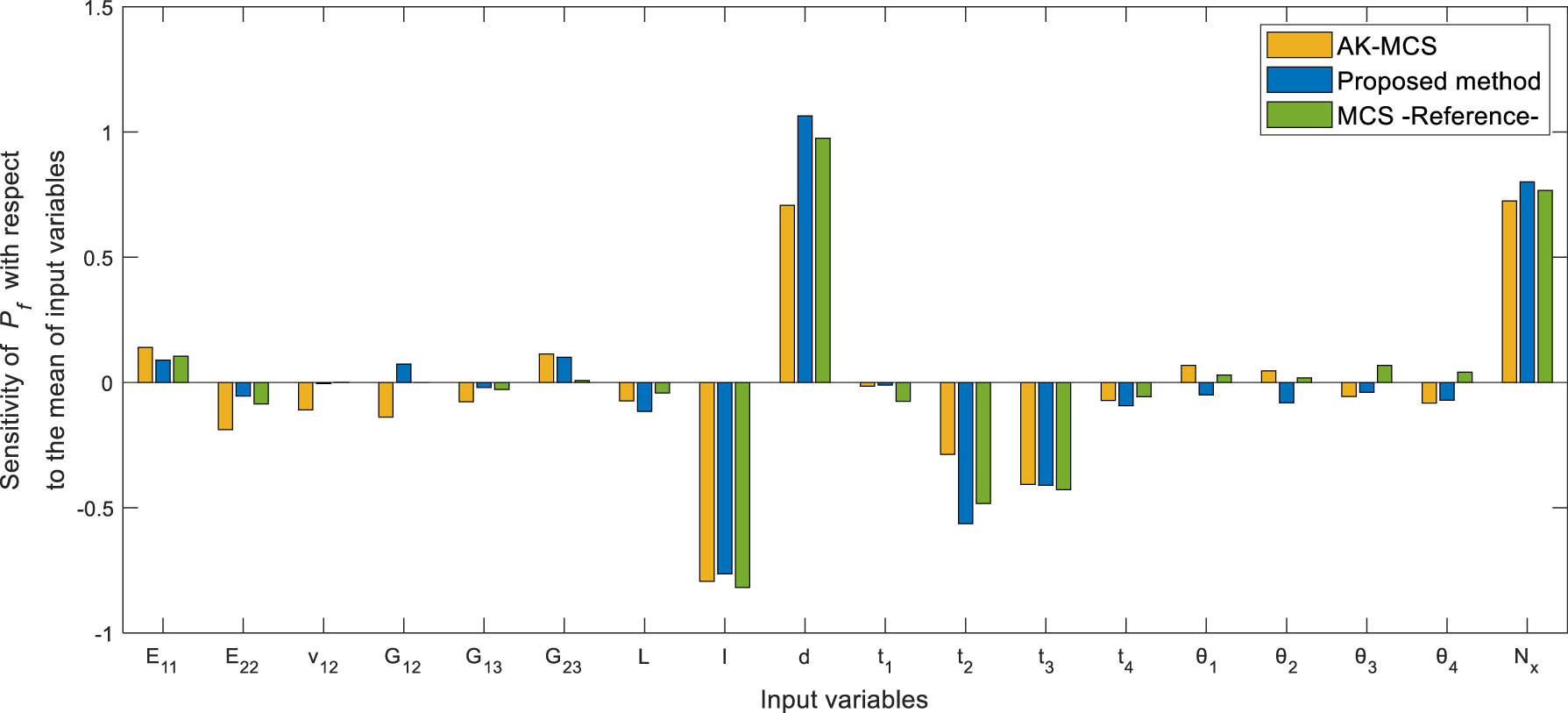
Sensitivity of failure probability to the mean of variables for example 1.

Sensitivity of failure probability to the standard deviation of variables for example 2.
As for the fiber orientation angles, they have no effect on the probability of failure when their mean changes. However, for variations in their standard deviations, angles θ 2 and θ 3 have an impact on the probability of failure. Finally, just like in the first example, the applied force has a substantial impact as a contributor to the probability of failure.
According to the results of our sensitivity analysis, to enhance the reliability and reduce the probability of failure of this composite plate, it is essential to decrease the hole diameter and increase the width of the composite, as these adjustments have a significant impact on the probability of failure. In addition, a slight increase in the thickness of the 90° oriented fiber layers can also contribute to strengthening the structure.
8 Conclusion
The new reliability methodology for laminated composites was presented, cleverly combining MCS with a metamodel resulting from the fusion of three approaches: ANN, SVM, and Kriging. This methodology demonstrated remarkable accuracy while minimizing the number of simulations required to estimate the probability of failure. Its efficiency is undeniable. However, it is important to note that the accuracy of the estimation may vary depending on the quality of the metamodels used, as shown in our second example where the precision of the metamodels slightly decreased. Thus, ensuring the robustness of the metamodels is essential to guarantee reliable results. It is important to emphasize that the failure criteria used in our analysis may not always accurately reflect the actual behavior of composite materials in complex situations. The accuracy of these criteria should be considered in the interpretation of the results.
In addition, local sensitivity was evaluated, highlighting the critical variables that most influence the probability of failure. This rigorous analysis has allowed us to recommend essential optimization measures to strengthen reliability and reduce the probability of failure of composite plates. In particular, it is imperative to prioritize the optimization of the thickness of the laminated layers, to choose high-quality composite materials, and to ensure that the dimensions strictly meet the required specifications. These actions aim to guarantee optimal performance of laminated composite materials, even in uncertain situations, and to strengthen their structural integrity.
In summary, this study opens valuable perspectives for improving design and decision-making in the field of laminated composite materials, while ensuring reliable performance in the face of uncertainty. It encourages further research to further refine the reliability and sensitivity methodologies applicable to these crucial materials in modern engineering.
-
Funding information: The authors state no funding involved.
-
Author contributions: All authors have accepted responsibility for the entire content of this manuscript and approved its submission.
-
Conflict of interest: The authors state no conflict of interest.
References
[1] Timoshenko S, Woinowsky-Krieger S. Theory of plates and shells. Vol. 2. New York: McGraw-hill; 1959.Search in Google Scholar
[2] Reddy JN. Theory and analysis of elastic plates and shells. Boca Raton: CRC Press; 2006.10.1201/9780849384165Search in Google Scholar
[3] Reddy JN. A refined nonlinear theory of plates with transverse shear deformation. Int J Solids Struct. 1984;20(9–10):881–96.10.1016/0020-7683(84)90056-8Search in Google Scholar
[4] Hosseini-Hashemi S, Fadaee M, Atashipour SR. Study on the free vibration of thick functionally graded rectangular plates according to a new exact closed-form procedure. Compos Struct. 2011;93(2):722–35.10.1016/j.compstruct.2010.08.007Search in Google Scholar
[5] Reddy JN. A refined shear deformation theory for the analysis of laminated plates. National Aeronautics and Space Administration; 1986.Search in Google Scholar
[6] Tornabene F, Viscoti M, Dimitri R. Generalized higher order layerwise theory for the dynamic study of anisotropic doubly -curved shells with a mapped geometry. Eng Anal Bound Elem. 2022;134:147–83.10.1016/j.enganabound.2021.09.017Search in Google Scholar
[7] Tornabene F, Viscoti M, Dimitri R. Static analysis of doubly-curved shell structures of smart materials and arbitrary shape subjected to general loads employing higher order theories and generalized differential quadrature method. Comput Model Eng Sci. 2022;133(3):719–98.10.32604/cmes.2022.022210Search in Google Scholar
[8] Brischetto S. Hygrothermal loading effects in bending analysis of multilayered composite plates. Comput Model Eng Sci (CMES). 2012 Nov;88(5):367–417.Search in Google Scholar
[9] Civalek Ö. Free vibration and buckling analyses of composite plates with straight-sided quadrilateral domain based on DSC approach. Finite Elem Anal Des. 2007;43(13):1013–22.10.1016/j.finel.2007.06.014Search in Google Scholar
[10] Abdo T, Rackwitz R. A new beta-point algorithm for large time-invariant and time-variant reliability problems. In: Der Kiureghian A, Thoft-Christensen P, editors. Reliability and Optimization of Structural Systems. Vol. 90. Berlin, Heidelberg: Springer; 1991. p. 1–12 (Lecture Notes in Engineering).10.1007/978-3-642-84362-4_1Search in Google Scholar
[11] Rackwitz R, Flessler B. Structural reliability under combined random load sequences. Comput Struct. 1978;9(5):489–94.10.1016/0045-7949(78)90046-9Search in Google Scholar
[12] Hartini E, Adrial H, Pujiarta S. Reliability analysis of primary and purification pumps in RSG-GAS using Monte Carlo simulation approach. J Teknol Reakt Nukl Tri Dasa Mega. 2019;21(1):15–22.10.17146/tdm.2019.21.1.5311Search in Google Scholar
[13] Au SK, Beck JL. A new adaptive importance sampling scheme for reliability calculations. Struct Saf. 1999;21(2):135–58.10.1016/S0167-4730(99)00014-4Search in Google Scholar
[14] Engelund S, Rackwitz R. A benchmark study on importance sampling techniques in structural reliability. Struct Saf. 1993;12(4):255–76.10.1016/0167-4730(93)90056-7Search in Google Scholar
[15] Ibrahim Y. Observations on applications of importance sampling in structural reliability analysis. Struct Saf. 1991;9(4):269–81.10.1016/0167-4730(91)90049-FSearch in Google Scholar
[16] Melchers RE. Importance sampling in structural systems. Struct Saf. 1989;6(1):3–10.10.1016/0167-4730(89)90003-9Search in Google Scholar
[17] Tokdar ST, Kass RE. Importance sampling: a review. WIREs Comput Stat. 2010;2(1):54–60.10.1002/wics.56Search in Google Scholar
[18] Au SK, Ching J, Beck JL. Application of subset simulation methods to reliability benchmark problems. Struct Saf. 2007;29(3):183–93.10.1016/j.strusafe.2006.07.008Search in Google Scholar
[19] Au SK, Beck JL. Estimation of small failure probabilities in high dimensions by subset simulation. Probab Eng Mech. 2001;16(4):263–77.10.1016/S0266-8920(01)00019-4Search in Google Scholar
[20] Bjerager P. Probability integration by directional simulation. J Eng Mech. 1988;114(8):1285–302.10.1061/(ASCE)0733-9399(1988)114:8(1285)Search in Google Scholar
[21] Nie J, Ellingwood BR. Directional methods for structural reliability analysis. Struct Saf. 2000;22(3):233–49.10.1016/S0167-4730(00)00014-XSearch in Google Scholar
[22] Zio E, Pedroni N. Functional failure analysis of a thermal–hydraulic passive system by means of line sampling. Reliab Eng Syst Saf. 2009;94(11):1764–81.10.1016/j.ress.2009.05.010Search in Google Scholar
[23] Pradlwarter HJ, Schuëller GI, Koutsourelakis PS, Charmpis DC. Application of line sampling simulation method to reliability benchmark problems. Struct Saf. 2007;29(3):208–21.10.1016/j.strusafe.2006.07.009Search in Google Scholar
[24] Bucher CG, Bourgund U. A fast and efficient response surface approach for structural reliability problems. Struct Saf. 1990;7(1):57–66.10.1016/0167-4730(90)90012-ESearch in Google Scholar
[25] Gavin HP, Yau SC. High-order limit state functions in the response surface method for structural reliability analysis. Struct Saf. 2008;30(2):162–79.10.1016/j.strusafe.2006.10.003Search in Google Scholar
[26] Huh J. Reliability analysis of nonlinear structural systems using response surface method. KSCE J Civ Eng. 2000;4(3):135–43.10.1007/BF02830867Search in Google Scholar
[27] Rajashekhar MR, Ellingwood BR. A new look at the response surface approach for reliability analysis. Struct Saf. 1993;12(3):205–20.10.1016/0167-4730(93)90003-JSearch in Google Scholar
[28] Deng J, Gu D, Li X, Yue ZQ. Structural reliability analysis for implicit performance functions using artificial neural network. Struct Saf. 2005;27(1):25–48.10.1016/j.strusafe.2004.03.004Search in Google Scholar
[29] Papadrakakis M, Papadopoulos V, Lagaros ND. Structural reliability analyis of elastic-plastic structures using neural networks and Monte Carlo simulation. Comput Methods Appl Mech Eng. 1996;136(1):145–63.10.1016/0045-7825(96)01011-0Search in Google Scholar
[30] Shao S, Murotsu Y. Structural reliability analysis using a neural network. JSME Int J Ser A. 1997;40(3):242–6.10.1299/jsmea.40.242Search in Google Scholar
[31] Dai HZ, Zhao W, Wang W, Cao ZG. An improved radial basis function network for structural reliability analysis. J Mech Sci Technol. 2011;25(9):2151–9.10.1007/s12206-011-0704-5Search in Google Scholar
[32] Deng J. Structural reliability analysis for implicit performance function using radial basis function network. Int J Solids Struct. 2006;43(11):3255–91.10.1016/j.ijsolstr.2005.05.055Search in Google Scholar
[33] Jing Z, Chen J, Li X. RBF-GA: An adaptive radial basis function metamodeling with genetic algorithm for structural reliability analysis. Reliab Eng Syst Saf. 2019;189:42–57.10.1016/j.ress.2019.03.005Search in Google Scholar
[34] Bichon BJ, Eldred MS, Swiler LP, Mahadevan S, McFarland JM. Efficient global reliability analysis for nonlinear implicit performance functions. AIAA J. 2008;46(10):2459–68.10.2514/1.34321Search in Google Scholar
[35] Kaymaz I. Application of kriging method to structural reliability problems. Struct Saf. 2005;27(2):133–51.10.1016/j.strusafe.2004.09.001Search in Google Scholar
[36] Vapnik VN. An overview of statistical learning theory. IEEE Trans Neural Netw. 1999;10(5):988–99.10.1109/72.788640Search in Google Scholar PubMed
[37] Vapnik V. The nature of statistical learning theory. Springer Science & Business Media; 1999. p. 340.10.1007/978-1-4757-3264-1Search in Google Scholar
[38] Onkar AK, Upadhyay CS, Yadav D. Probabilistic failure of laminated composite plates using the stochastic finite element method. Compos Struct. 2007;77(1):79–91.10.1016/j.compstruct.2005.06.006Search in Google Scholar
[39] Lopes PAM, Gomes HM, Awruch AM. Reliability analysis of laminated composite structures using finite elements and neural networks. Compos Struct. 2010;92(7):1603–13.10.1016/j.compstruct.2009.11.023Search in Google Scholar
[40] Dey S, Mukhopadhyay T, Sahu SK, Li G, Rabitz H, Adhikari S. Thermal uncertainty quantification in frequency responses of laminated composite plates. Compos Part B Eng. 2015;80:186–97.10.1016/j.compositesb.2015.06.006Search in Google Scholar
[41] Chen W, Jia P. Interlaminar stresses analysis and the limit state function approximating methods for composite structure reliability assessment: A selected review and some perspectives. J Compos Mater. 2013;47(12):1535–47.10.1177/0021998312449676Search in Google Scholar
[42] Momeni Badeleh M, Fallah NA. Probabilistic reliability analysis for active vibration control of piezoelectric laminated composite plates using mesh-free finite volume method. J Intell Mater Syst Struct. 2023;34(7):836–60.10.1177/1045389X221121945Search in Google Scholar
[43] Martinez JR, Bishay PL, Tawfik ME, Sadek EA. Reliability analysis of smart laminated composite plates under static loads using artificial neural networks. Heliyon. 2022;8(12):e11889.10.1016/j.heliyon.2022.e11889Search in Google Scholar PubMed PubMed Central
[44] Haeri A, Fadaee MJ. Efficient reliability analysis of laminated composites using advanced Kriging surrogate model. Compos Struct. 2016;149:26–32.10.1016/j.compstruct.2016.04.013Search in Google Scholar
[45] Mathew TV, Prajith P, Ruiz RO, Atroshchenko E, Natarajan S. Adaptive importance sampling based neural network framework for reliability and sensitivity prediction for variable stiffness composite laminates with hybrid uncertainties. Compos Struct. 2020;245:112344.10.1016/j.compstruct.2020.112344Search in Google Scholar
[46] Zhou C, Li C, Zhang H, Zhao H, Zhou C. Reliability and sensitivity analysis of composite structures by an adaptive Kriging based approach. Compos Struct. 2021;278:114682.10.1016/j.compstruct.2021.114682Search in Google Scholar
[47] Morio J. Global and local sensitivity analysis methods for a physical system. Eur J Phys. 2011;32(6):1577.10.1088/0143-0807/32/6/011Search in Google Scholar
[48] Wu YT. Computational methods for efficient structural reliability and reliability sensitivity analysis. AIAA J. 1994;32(8):1717–23.10.2514/3.12164Search in Google Scholar
[49] Wei P, Tang C, Yang Y. Structural reliability and reliability sensitivity analysis of extremely rare failure events by combining sampling and surrogate model methods. Proc Inst Mech Eng Part O J Risk Reliab. 2019;233(6):943–57.10.1177/1748006X19844666Search in Google Scholar
[50] Kaw AK. Mechanics of composite materials. Boca Raton: CRC Press; 2005. p. 491.10.1201/9781420058291Search in Google Scholar
[51] Beltrami E. Sulle condizioni di resistenza dei corpi elastici. Il Nuovo Cimento. 1885;18(1):145–55.10.1007/BF02824697Search in Google Scholar
[52] Wang Z, Shafieezadeh A. REAK: Reliability analysis through Error rate-based Adaptive Kriging. Reliab Eng Syst Saf. 2019;182:33–45.10.1016/j.ress.2018.10.004Search in Google Scholar
[53] Echard B, Gayton N, Lemaire M. AK-MCS: An active learning reliability method combining Kriging and Monte Carlo simulation. Struct Saf. 2011;33(2):145–54.10.1016/j.strusafe.2011.01.002Search in Google Scholar
[54] Wu YT, Mohanty S. Variable screening and ranking using sampling-based sensitivity measures. Reliab Eng Syst Saf. 2006;91(6):634–47.10.1016/j.ress.2005.05.004Search in Google Scholar
[55] Martinez JR, Bishay PL. On the stochastic first-ply failure analysis of laminated composite plates under in-plane tensile loading. Compos Part C Open Access. 2021;4:100102.10.1016/j.jcomc.2020.100102Search in Google Scholar
[56] Amrane C, Mattrand C, Beaurepaire P, Bourinet JM, Gayton N. On the use of ensembles of metamodels for estimation of the failure probability. In: Proceedings of the 3rd International Conference on Uncertainty Quantification in Computational Sciences and Engineering (UNCECOMP 2019); 2019 June 24–26; Crete, Greece: Institute of Structural Analysis and Antiseismic Research School of Civil Engineering National Technical University of Athens (NTUA) Greece; 2019. p. 343–56.10.7712/120219.6345.18430Search in Google Scholar
[57] Cheng K, Lu Z. Structural reliability analysis based on ensemble learning of surrogate models. Struct Saf. 2020;83:101905.10.1016/j.strusafe.2019.101905Search in Google Scholar
[58] Goel T, Haftka RT, Shyy W, Queipo NV. Ensemble of surrogates. Struct Multidiscip Optim. 2007;33(3):199–216.10.1007/s00158-006-0051-9Search in Google Scholar
[59] Hoeting JA, Madigan D, Raftery AE, Volinsky CT. Bayesian model averaging: a tutorial with comments by M. Clyde, David Draper and E. I. George, and a rejoinder by the authors. Stat Sci. 1999;14(4):382–417.10.1214/ss/1009212519Search in Google Scholar
[60] Zerpa LE, Queipo NV, Pintos S, Salager JL. An optimization methodology of alkaline–surfactant–polymer flooding processes using field scale numerical simulation and multiple surrogates. J Pet Sci Eng. 2005;47(3):197–208.10.1016/j.petrol.2005.03.002Search in Google Scholar
[61] Rafiq MY, Bugmann G, Easterbrook DJ. Neural network design for engineering applications. Comput Struct. 2001;79(17):1541–52.10.1016/S0045-7949(01)00039-6Search in Google Scholar
[62] Karush W. Minima of functions of several variables with inequalities as side conditions. Department of Mathematics, University of Chicago; 1939.Search in Google Scholar
[63] Matheron G. The intrinsic random functions and their applications. Adv Appl Probab. 1973;5(3):439–68.10.2307/1425829Search in Google Scholar
[64] Sacks J, Schiller SB, Welch WJ. Designs for computer experiments. Technometrics. 1989;31(1):41–7.10.1080/00401706.1989.10488474Search in Google Scholar
[65] Reddy J, Pandey A. A first-ply failure analysis of composite laminates. Comput Struct. 1987;25(3):371–93.10.1016/0045-7949(87)90130-1Search in Google Scholar
[66] Reddy Y, Reddy J. Linear and non-linear failure analysis of composite laminates with transverse shear. Compos Sci Technol. 1992;44(3):227–55.10.1016/0266-3538(92)90015-USearch in Google Scholar
© 2024 the author(s), published by De Gruyter
This work is licensed under the Creative Commons Attribution 4.0 International License.
Articles in the same Issue
- Research Articles
- Flutter investigation and deep learning prediction of FG composite wing reinforced with carbon nanotube
- Experimental and numerical investigation of nanomaterial-based structural composite
- Optimisation of material composition in functionally graded plates for thermal stress relaxation using statistical design support system
- Tensile assessment of woven CFRP using finite element method: A benchmarking and preliminary study for thin-walled structure application
- Reliability and sensitivity assessment of laminated composite plates with high-dimensional uncertainty variables using active learning-based ensemble metamodels
- Performances of the sandwich panel structures under fire accident due to hydrogen leaks: Consideration of structural design and environment factor using FE analysis
- Recycling harmful plastic waste to produce a fiber equivalent to carbon fiber reinforced polymer for reinforcement and rehabilitation of structural members
- Effect of seed husk waste powder on the PLA medical thread properties fabricated via 3D printer
- Finite element analysis of the thermal and thermo-mechanical coupling problems in the dry friction clutches using functionally graded material
- Strength assessment of fiberglass layer configurations in FRP ship materials from yard practices using a statistical approach
- An enhanced analytical and numerical thermal model of frictional clutch system using functionally graded materials
- Using collocation with radial basis functions in a pseudospectral framework to the analysis of laminated plates by the Reissner’s mixed variational theorem
- A new finite element formulation for the lateral torsional buckling analyses of orthotropic FRP-externally bonded steel beams
- Effect of random variation in input parameter on cracked orthotropic plate using extended isogeometric analysis (XIGA) under thermomechanical loading
- Assessment of a new higher-order shear and normal deformation theory for the static response of functionally graded shallow shells
- Nonlinear poro thermal vibration and parametric excitation in a magneto-elastic embedded nanobeam using homotopy perturbation technique
- Finite-element investigations on the influence of material selection and geometrical parameters on dental implant performance
- Study on resistance performance of hexagonal hull form with variation of angle of attack, deadrise, and stern for flat-sided catamaran vessel
- Evaluation of double-bottom structure performance under fire accident using nonlinear finite element approach
- Behavior of TE and TM propagation modes in nanomaterial graphene using asymmetric slab waveguide
- FEM for improvement of damage prediction of airfield flexible pavements on soft and stiff subgrade under various heavy load configurations of landing gear of new generation aircraft
- Review Article
- Deterioration and imperfection of the ship structural components and its effects on the structural integrity: A review
- Erratum
- Erratum to “Performances of the sandwich panel structures under fire accident due to hydrogen leaks: Consideration of structural design and environment factor using FE analysis”
- Special Issue: The 2nd Thematic Symposium - Integrity of Mechanical Structure and Material - Part II
- Structural assessment of 40 ft mini LNG ISO tank: Effect of structural frame design on the strength performance
- Experimental and numerical investigations of multi-layered ship engine room bulkhead insulation thermal performance under fire conditions
- Investigating the influence of plate geometry and detonation variations on structural responses under explosion loading: A nonlinear finite-element analysis with sensitivity analysis