Asymmetric Auctions with Discretely Distributed Valuations

3.1 Equilibrium Bidding in the First Price Auction

In the first price auction, FPA henceforth, each bidder simultaneously submits a sealed bid, the highest bidder wins and pays his bid to the seller. For some tie-breaking rules, no pure-strategy equilibrium exists in this game, but Proposition 2 in Maskin and Riley (2000b) establishes that an equilibrium, possibly in mixed strategies, exists under the “Vickrey tie-breaking rule”, according to which each bidder i is required to submit both an “ordinary” bid b _i ≥ 0 and a “tie-breaker” bid c _i ≥ 0.^[8] The tie-breaking rule (see Maskin and Riley 2000b for a complete description) specifies that c ₁, c ₂ matter only when b ₁ = b ₂, and implies that for each bidder i it is weakly dominant to choose c _i equal to v _i − b _i . Hence, in describing a strategy of bidder i, to each b _i we implicitly associate c _i = v _i − b _i . As a result, when b ₁ = b ₂ the bidder with the highest value wins and pays to the seller the other bidder’s value. Proposition 1 below identifies, for each parameter values, a unique equilibrium for the FPA under the Vickrey tie-breaking rule.

We use i _j to denote type j of bidder i, for j = L, M, H and i = 1, 2, and as a notation for mixed strategies we let G _ij denote the c.d.f. of the (ordinary) bid submitted by type i _j ; u i j F is type i _j ’s equilibrium expected utility. In order to fix the ideas, without loss of generality we assume

This means that bidder 1 is ex ante weakly stronger than bidder 2 in the sense that Pr{v ₁ = v _H } is no less than Pr{v ₂ = v _H }, a condition weaker than first order stochastic dominance.

Arguing as in Maskin and Riley (1985) and in Riley (1989), we deduce that each Bayes Nash Equilibrium is such that for i = 1, 2, type i _L bids v _L with probability 1 (a pure strategy), the set of possible realizations of G _iM is an interval [ v L , b ̄ i M ] in which b ̄ i M may be equal to v _L , the set of possible realizations of G _iH is an interval [ b ̄ i M , b ̄ i H ] in which b ̄ i M < b ̄ i H (with no probability mass on a single bid different from v _L ), and b ̄ 1 H = b ̄ 2 H . In the following, b ̄ H denotes both b ̄ 1 H and b ̄ 2 H .

In order to determine the mixed strategy G _ij for each type i _j , we define G _i (b) as λ _i G _iL (b) + μ _i G _iM (b) + η _i G _iH (b), that is G _i is the c.d.f. of the bids submitted by bidder i. In equilibrium, type i _j is indifferent among all the bids in the set of the possible realizations of G _ij . In particular, for type 1 _M the equality ( v M − b ) G 2 ( b ) = u 1 M F holds for each b ∈ ( v L , b ̄ 1 M ] , and u 1 M F coincides with lim b ↓ v L ( v M − b ) G 2 ( b ) , that is with G ₂(v _L )Δ. We know that G ₂(v _L ) ≥ λ ₂ since type 2 _L bids v _L , but we cannot rule out that also type 2 _M bids v _L with positive probability. Hence G ₂(v _L ) may be greater than λ ₂, and we use ρ ₂ to denote G ₂(v _L ); likewise, we set ρ ₁ = G ₁(v _L ). Therefore^[9]

The indifference conditions for types 1 _M , 1 _H , 2 _M , 2 _H yield the following equalities, in which v H − b ̄ H = u 1 H F = u 2 H F :

We prove below that in our setting with three types for each bidder, sometimes it is bidder 1 who bids v _L with probability ρ ₁ greater than λ ₁, sometimes it is bidder 2 who bids v _L with probability ρ ₂ > λ ₂.

In order to derive G ₁, G ₂ from (3) to (6), we need to determine b ̄ 1 M , b ̄ 2 M , b ̄ H , ρ 1 , ρ 2 .^[11] Next lemma shows that (1) implies b ̄ 1 M ≤ b ̄ 2 M , hence type 1 _H (type 1 _M ) is less aggressive in terms of the set of possible bids than type 2 _H (than type 2 _M ).^[12]

It turns out that b ̄ 1 M > v L for some parameter values, but b ̄ 1 M = v L for other parameter values. In the first case, from (3) to (6) it follows that

In the second case, (7) still applies to b ̄ 2 M , b ̄ H , but the first equality in (7) is replaced by b ̄ 1 M = v L .

For each parameter values, Proposition 1 determines ρ ₁, ρ ₂ uniquely, thus identifies a unique equilibrium, which is one of the following three strategy profiles:

In each of these profiles, types 1 _L and 2 _L both bid v _L . The profiles mainly differ because of the additional bidder types who bid v _L with positive probability: in P _2M it is only type 2 _M ; in P _1M it is only type 1 _M ; in P _1MH , both type 1 _M (with probability 1) and type 1 _H bid v _L with positive probability. Notice from (10) that in P _1MH bidding is not affected by λ ₁, μ ₁.

By Proposition 1, there exist three different equilibrium regimes, (8)–(10), and (11), (12) determine the regime which applies. Figures 1a and 1b below provide a graphical illustration of Proposition 1 by fixing λ ₂, μ ₂ and representing the space of (λ ₁, μ ₁) which satisfy (1), that is the triangle with bold edges and vertices (0,0), (λ ₂ + μ ₂, 0), (0, λ ₂ + μ ₂); the point (λ ₁, μ ₁) = (λ ₂, μ ₂) is on the hypothenuse of this triangle.

Figure 1a:

The regions R _1M , R _2M  when λ ₂ ≤ μ ₂.

Figure 1a refers to the case with λ ₂ ≤ μ ₂, which makes (12) satisfied for each (λ ₁, μ ₁), hence P _1M or P _2M is the equilibrium: Region R _2M is the set of (λ ₁, μ ₁) for which (11) holds and P _2M is the equilibrium; R _1M is the region in which (11) is violated and P _1M is the equilibrium. The curve C, connecting point (0,0) to (λ ₂, μ ₂), is the set of (λ ₁, μ ₁) such that (11) is an equality, which implies (ρ ₁, ρ ₂) = (λ ₁, λ ₂) and only types 1 _L , 2 _L bid v _L .

Figure 1b is about the case of λ ₂ > μ ₂. Then there exist (λ ₁, μ ₁) close to (0,0) which violate (12) and R _1MH is the region consisting of such (λ ₁, μ ₁); P _1MH is the equilibrium for each (λ ₁, μ ₁) ∈ R _1MH . In P _1MH , type 1 _H bids v _L with positive probability and we notice that this may occur only if λ ₂ > μ ₂ because 1 _H ’s utility from bidding v _L is 2λ ₂Δ, but by bidding v _M , type 1 _H wins with probability greater than λ ₂ + μ ₂, earning utility greater than (λ ₂ + μ ₂)Δ. Thus λ ₂ ≤ μ ₂ makes the bid v _L less profitable than the bid v _M , and rules out that 1 _H bids v _L . This is why P _1MH is never an equilibrium when λ ₂ ≤ μ ₂.

Figure 1b:

The regions R _1M , R _2M , R _1MH when λ ₂ > μ ₂.

The expected revenue R ^F in the FPA is the expectation of the highest bid, which is equal to v _L with probability ρ ₁ ρ ₂ and has c.d.f. G ₁(b)G ₂(b) for b ∈ ( v L , b ̄ H ] , with G ₁(b), G ₂(b) determined by (3)–(6):

On the Effects of Asymmetry on Bidding in the FPA The literature on asymmetric auctions mainly focuses on settings with two bidders and provides sufficient conditions on the c.d.f.s for the bidders’ values to draw conclusions about the comparison between the bidders’ equilibrium bidding, for instance one bidder’s bid distribution is stronger than the other bidder’s. In our setting, Ceesay, Doni, Menicucci (2024) use Proposition 1 to show that the comparison results can be proved under conditions which are typically weaker than the literature’s conditions, and to examine the effects of asymmetry on bidding.

3.2 Equilibrium Bidding in the Second Price Auction

In the second price auction, SPA henceforth, for each bidder it is weakly dominant to bid the own valuation. We use u i j S to denote the expected utility of type i _j , for j = L, M, H, i = 1, 2. Hence u 1 L S = u 2 L S = 0 and

The expected revenue R ^S in the SPA is the expectation of the second highest valuation, that is R ^S = v _L + (μ ₁ μ ₂ + μ ₁ η ₂ + η ₁ μ ₂)Δ + 2η ₁ η ₂Δ, and after simple manipulations it can be written as

4.1 Comparison of Rents

It is immediate from (2) and (13) that both type 1 _M and 2 _M weakly prefer the FPA, that is u 1 M F ≥ u 1 M S and u 2 M F ≥ u 2 M S , since ρ ₂ ≥ λ ₂ and ρ ₁ ≥ λ ₁ (with one strict inequality unless (11) is an equality). This occurs because in the FPA type 1 _M or type 2 _M bids v _L with positive probability, which makes type 2 _M or type 1 _M better off than in the SPA.

The same preference holds for type 2 _H , that is u 2 H F ≥ u 2 H S , because in the FPA type 2 _H benefits from b ̄ 1 M < b ̄ 2 M , that is type 1 _H bids below b ̄ 2 M with positive probability. Hence type 1 _H loses with positive probability against b ̄ 2 M , the highest bid submitted by type 2 _M , and when bidding b ̄ 2 M , type 2 _H beats types 1 _L , 1 _M for sure, and also type 1 _H with positive probability. Thus 2 _H wins with probability greater than λ ₁ + μ ₁. Conversely, under the SPA type 2 _H wins and earns a positive utility only when facing type 1 _L or 1 _M , that is with probability λ ₁ + μ ₁.

Matters are different for type 1 _H , because u 1 H F is equal to u 2 H F , but u 1 H S = ( 2 λ 2 + μ 2 ) Δ may be higher than u 2 H S = ( 2 λ 1 + μ 1 ) Δ ; next lemma identifies precisely when u 1 H F < u 1 H S holds.

By Lemma 2, only type 1 _H may prefer the SPA to the FPA, hence it is intuitive that U ^F ≥ U ^S , and therefore R ^F < R ^S , hold frequently. In particular, when λ ₁ ≥ λ ₂ each bidder type weakly prefers the FPA to the SPA, hence U ^F > U ^S if λ ₁ ≥ λ ₂. We state this result in Proposition 2 below, jointly with another sufficient condition for U ^F > U ^S . We remark that this goes in the opposite direction with respect to most of the literature, which finds that the revenue under the FPA is higher than under the SPA.

However, the opposite inequalities U ^F < U ^S and R ^F > R ^S hold for some parameter values, for instance if λ 1 = 1 5 , μ 1 = 1 10 and λ 2 = μ 2 = 2 5 . Then U ^F = 1.02 < U ^S = 1.06 and R ^F = 0.6214 > R ^S = 0.62.^[14] In next subsection we investigate more deeply the comparison between R ^F and R ^S .

4.2 Comparison of Revenues

In this subsection we focus on the direct comparison between R ^F and R ^S . Since Lemma 2 suggests that R ^F < R ^S often holds, we perform the comparison by fixing (λ ₂, μ ₂) and inquiring whether there exist (λ ₁, μ ₁) such that R ^F > R ^S , or if instead R ^F ≤ R ^S for each (λ ₁, μ ₁) which satisfies (1). We denote with F ₂ the set of (λ ₂, μ ₂) such that R ^F > R ^S for some (λ ₁, μ ₁), and with S ₂ the (complementary) set of (λ ₂, μ ₂) such that R ^F ≤ R ^S for each (λ ₁, μ ₁). In determining F ₂ and S ₂, Proposition 2 below distinguishes the case of λ ₂ ≤ μ ₂ from the case of λ ₂ > μ ₂ because in the first case two equilibrium regimes exist, P _1M and P _2M , whereas in the second case a third equilibrium regime exists, P _1MH .

Proposition 2 establishes that given (λ ₂, μ ₂), in order to determine whether there exist (λ ₁, μ ₁) such that R ^F > R ^S it suffices to evaluate R ^F − R ^S at a specific (λ ₁, μ ₁) – which we argue below induces the most aggressive bidding in the FPA. As a result, the sets F ₂ and S ₂ are identified: F ₂ consists of all (λ ₂, μ ₂) which satisfy λ ₂ ≤ μ ₂ and (15), or λ ₂ > μ ₂ and (16), and is the grey set in Figure 2; S ₂ is the white set in Figure 2, and by Corollary 1 it includes each (λ ₂, μ ₂) such that λ 2 + μ 2 ≤ 1 2 .^[15]

Figure 2:

The set of (λ ₂, μ ₂) which satisfy (15) when λ ₂ ≤ μ ₂, or (16) when λ ₂ > μ ₂.

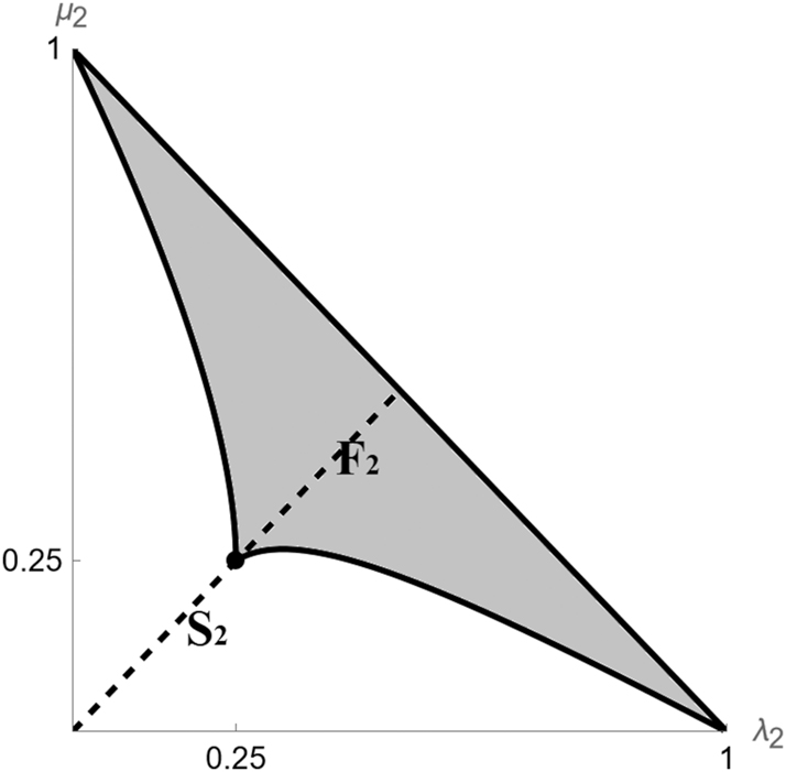
The case of λ ₂ ≤ μ ₂ In the following, for ease of language, instead of (λ ₁, μ ₁) close to (0,0) we write (λ ₁, μ ₁) = (0, 0). When λ ₂ ≤ μ ₂, Proposition 2(i) establishes that there exist (λ ₁, μ ₁) such that R ^F > R ^S if and only if R ^F > R ^S holds when (λ ₁, μ ₁) = (0, 0), and such condition is equivalent to (15).

We remark that (λ ₁, μ ₁) = (0, 0) induces the most aggressive bidding in the FPA, given λ ₂ ≤ μ ₂, because (3)–(6), (7) reveal that G ₁, G ₂ are more aggressive the lower are ρ ₁, ρ ₂. Precisely, ρ ₁ ≥ λ ₁, ρ ₂ ≥ λ ₂ by (2) and (λ ₁, μ ₁) = (0, 0) implies ρ ₁ = 0, ρ ₂ = λ ₂, which are the lowest possible values for ρ ₁, ρ ₂ given λ ₂, μ ₂. But we stress that (λ ₁, μ ₁) = (0, 0) alone is not sufficient for R ^F > R ^S to hold: (λ ₁, μ ₁) = (0, 0) induces the most aggressive bidding also in the SPA, and the sign of R ^F − R ^S when (λ ₁, μ ₁) = (0, 0) is determined by whether (15) is satisfied, which occurs if and only if μ 2 ≥ 1 4 and λ ₂ is large enough given λ ₂ ≤ μ ₂. We explain below why R ^F > R ^S when these conditions hold.

First notice that when λ ₁, μ ₁ are about 0, bidder 1 almost certainly has value v _H and there are three relevant states of the world: (v ₁, v ₂) equal to (v _H , v _L ), or equal to (v _H , v _M ), or equal to (v _H , v _H ). From (7) we see that b ̄ 2 M is close to v _M , and (5) implies that G ₁(b) is close to 0 for each b < v _M , that is in the limit as (λ ₁, μ ₁) → (0, 0), G ₁ puts all the probability on bids no less than v _M . In other words, bidder 1 (i.e. type 1 _H ) bids at least v _M ;^[16] hence the revenue under the FPA is greater than v _M . Conversely, under the SPA the revenue coincides with v ₂ in each state mentioned above as min{v ₁, v ₂} = min{v _H , v ₂} = v ₂. Hence the revenue is greater in the FPA when (v ₁, v ₂) = (v _H , v _L ) or (v ₁, v ₂) = (v _H , v _M ), but is greater in the SPA when (v ₁, v ₂) = (v _H , v _H ). This makes it intuitive that R ^F > R ^S if λ ₂ is large, as the greater is λ ₂, the greater is the probability of state (v _H , v _L ), in which the FPA has a higher revenue, and the lower is the probability of state (v _H , v _H ), in which the SPA has a greater revenue. In particular, R ^F > R ^S if λ ₂ is close to 1 − μ ₂ because then (v _H , v _H ), the only state in which the SPA is superior to the FPA, has probability about zero.

The case of λ ₂ > μ ₂ When λ ₂ > μ ₂, Proposition 2(ii) establishes a result analogous to Proposition 2(i), that is R ^F > R ^S holds for some (λ ₁, μ ₁) if and only if R ^F > R ^S when (λ ₁, μ ₁) = (λ ₂ − μ ₂, 0), and such condition is equivalent to (16). In a sense, now (λ ₁, μ ₁) = (λ ₂ − μ ₂, 0) plays the role (λ ₁, μ ₁) = (0, 0) plays when λ ₂ ≤ μ ₂. In order to see why, notice that (λ ₁, μ ₁) = (λ ₂ − μ ₂, 0) is a distribution of v ₁ which induces the most aggressive bidding in the FPA, given λ ₂ > μ ₂, because when (λ ₁, μ ₁) = (λ ₂ − μ ₂, 0) we have ρ ₂ = λ ₂ (this is the minimum value for ρ ₂) and ρ ₁ = λ ₂ − μ ₂, and for each other (λ ₁, μ ₁), ρ ₁ is greater than λ ₂ − μ ₂. Actually, any other (λ ₁, μ ₁) ∈ R _1MH induces the same bidding in the FPA like (λ ₁, μ ₁) = (λ ₂ − μ ₂, 0), as from Subsection 3.1 we know that if (λ ₁, μ ₁) ∈ R _1MH , then (12) is violated and R ^F is constant with respect to λ ₁, μ ₁. But R ^S in (14) is decreasing in λ ₁, μ ₁ with ∂ R S ∂ λ 1 < ∂ R S ∂ μ 1 < 0 . Hence (λ ₁, μ ₁) = (λ ₂ − μ ₂, 0) is the maximum point for R ^F − R ^S in R _1MH .

However, R ^F > R ^S at (λ ₁, μ ₁) = (λ ₂ − μ ₂, 0) if and only if (16) is satisfied, which is equivalent to λ 2 > 1 4 and μ ₂ sufficiently large, given λ ₂ > μ ₂. We explain in the following why R ^F > R ^S if these conditions are satisfied. When 1 4 < λ 2 ≤ 1 2 we have that μ ₂ large implies μ ₂ close to λ ₂, which is a setting close to one covered when λ ₂ ≤ μ ₂, for which we know that R ^F > R ^S . When λ 2 > 1 2 , we first describe the effect of an increase in μ ₂ on R ^F and on R ^S . An increase in μ ₂ increases R ^F as G ₂ is unchanged but G ₁ improves: see (3)–(6), (7) with ρ ₁ = λ ₁ = λ ₂ − μ ₂, ρ ₂ = λ ₂, μ ₁ = 0. An increase in μ ₂ has ambiguous net effect on R ^S as it reduces η ₂ (a negative effect) but it also decreases λ ₁ and increases η ₁ (a positive effect). However, when μ ₂ is close to its largest value 1 − λ ₂, the event v ₂ = v _H has a small probability and then the positive effect on R ^S due to the increase in η ₁ is small. As a result, the net effect is negative. Hence an increase in μ ₂ increases R ^F − R ^S and makes R ^F − R ^S positive when μ ₂ is close to 1 − λ ₂.

Figure 3a represents in grey, for a case in which λ ₂ ≤ μ ₂ and (15) holds, the set of (λ ₁, μ ₁) such that R ^F > R ^S . Figure 3b represents in grey the analogous set for a case in which λ ₂ > μ ₂ and (16) holds. In either case, the white set of (λ ₁, μ ₁) such that R ^F < R ^S includes each (λ ₁, μ ₁) such that λ ₁ ≥ λ ₂ or such that μ ₁ is large, consistently with Proposition 2(i–ii). In particular, these conditions imply R ^F < R ^S when (λ ₁, μ ₁) is close to (λ ₂, μ ₂), (λ ₁, μ ₁) ≠ (λ ₂, μ ₂).^[17]

Figure 3a:

The set of (λ ₁,t μ ₁) such that R ^F > R ^S  when λ ₂ = 0.4, μ ₂ = 0.5.

Figure 3b:

The set of (λ ₁, μ ₁) such that R ^F > R ^S  when λ ₂ = 0.6, μ ₂ = 0.3.

The Difference with the Setting with Binary Support At the beginning of Section 4 we have remarked that R ^F < R ^S when the support for each bidder’s value is {v _L , v _H }, that is when μ ₁ = μ ₂ = 0, for each λ ₁ < λ ₂. Conversely, Proposition 2 shows that R ^F > R ^S in some cases when the support is {v _L , v _M , v _H }.

In order to explain this difference, start from a symmetric setting with support {v _L , v _M , v _H } and 0 < μ ₁ = μ ₂ < λ ₁ = λ ₂; ^[18] thus R ^F = R ^S . Then consider a change in (λ ₁, μ ₁) from (λ ₁, μ ₁) = (λ ₂, μ ₂) to (λ ₁, μ ₁) = (λ ₂ − μ ₂, 0): see Figure 1b. This reduces ρ ₁ = λ ₁ and leaves ρ ₂ = λ ₂ unchanged, hence improves bidding in the FPA and increases R ^F . But it improves bidding also in the SPA and increases R ^S . Hence it is uncertain whether R ^F > R ^S at (λ ₁, μ ₁) = (λ ₂ − μ ₂, 0); this is determined by whether (16) is satisfied. The main point is that the considered improvement in the distribution of v ₁ increases both R ^F and R ^S .

Matters are different when the support is binary because μ ₂ = 0 implies that the set of (λ ₁, μ ₁) which satisfy (1) consists entirely of region R _1MH (while R _1M , R _2M are both empty). Then, when μ ₁ = μ ₂ = 0, a reduction in λ ₁ below λ ₂ keeps (λ ₁, μ ₁) in region R _1MH , in which bidding in the FPA does not depend on (λ ₁, μ ₁). Hence R ^F < R ^S for any λ ₁ < λ ₂ because when the distribution of v ₁ becomes stronger, R ^S increases but R ^F remains constant (as type 1 _H puts a probability mass on the bid v _L when λ ₁ < λ ₂). This feature of the FPA when the support is binary is responsible for the difference between the two settings.

Shift and Stretch Maskin and Riley (2000a) consider a few particular classes of asymmetries, one of which is called shift, another is called stretch. The shift asymmetry is such that the distribution of v ₁ is given by the distribution of v ₂ shifted to the right by a fixed positive amount. The stretch asymmetry is such that the distribution of v ₁ is a rightward stretch of the distribution of v ₂. In a setting with continuously distributed values, Maskin and Riley (2000a) prove that the FPA produces a higher revenue than the SPA for any shift and any stretch, under suitable assumptions on the distribution of v ₂ which is then shifted or stretched [Kirkegaard (2012) proves these results under slightly weaker assumptions]. Ceesay, Doni, Menicucci (2024) prove that in our context with three types, a significantly more nuanced picture emerges as R ^F < R ^S in a variety of cases.

References

Arozamena, L., and E. Cantillon. 2004. “Investment Incentives in Procurement Auctions.” The Review of Economic Studies 71 (1): 1–18. https://doi.org/10.1111/0034-6527.00273.Search in Google Scholar
Ceesay, M., N. Doni, and D. Menicucci. 2024. “Asymmetric Auctions with Discretely Distributed Valuations.” Department of Economics and Management of the University of Florence Working Paper n. 20/2024. https://www.disei.unifi.it/cmpro-v-p-95.html (accessed September 26, 2024).Search in Google Scholar
Cheng, H. 2006. “Ranking Sealed High-Bid and Open Asymmetric Auctions.” Journal of Mathematical Economics 42 (4–5): 471–98. https://doi.org/10.1016/j.jmateco.2006.05.008.Search in Google Scholar
Cheng, H. 2011. “Asymmetry and Revenue in First-Price Auctions.” Economics Letters 111 (1): 78–80. https://doi.org/10.1016/j.econlet.2010.12.004.Search in Google Scholar
Doni, N., and D. Menicucci. 2013. “Revenue Comparison in Asymmetric Auctions with Discrete Valuations.” The B.E. Journal of Theoretical Economics 13 (1): 429–61. https://doi.org/10.1515/bejte-2012-0014.Search in Google Scholar
Fibich, G., A. Gavious, and A. Sela. 2002. “Low and High Types in Asymmetric First-Price Auctions.” Economics Letters 75 (2): 283–7. https://doi.org/10.1016/S0165-1765(01)00611-5.Search in Google Scholar
Gavious, A., and Y. Minchuk. 2014. “Ranking Asymmetric Auctions.” International Journal of Game Theory 43: 369–93. https://doi.org/10.1007/s00182-013-0383-9.Search in Google Scholar
Kaplan, T. R., and S. Zamir. 2012. “Asymmetric First Price Auctions with Uniform Distributions: Analytical Solutions to the General Case.” Economic Theory 50: 269–302. https://doi.org/10.1007/s00199-010-0563-9.Search in Google Scholar
Kirkegaard, R. 2012. “A Mechanism Design Approach to Ranking Asymmetric Auctions.” Econometrica 80 (5): 2349–64. https://doi.org/10.3982/ECTA9859.Search in Google Scholar
Kirkegaard, R. 2014. “Ranking Asymmetric Auctions: Filling the Gap between a Distributional Shift and Stretch.” Games and Economic Behavior 85: 60–9. https://doi.org/10.1016/j.geb.2014.01.016.Search in Google Scholar
Kirkegaard, R. 2021. “Ranking Reversals in Asymmetric Auctions.” Journal of Mathematical Economics 95: 102478. https://doi.org/10.1016/j.jmateco.2021.102478.Search in Google Scholar
Lebrun, B. 2002. “Continuity of the First-Price Auction Nash Equilibrium Correspondence.” Economic Theory 20: 435–53. https://doi.org/10.1007/s001990100227.Search in Google Scholar
Li, H., and J. Riley. 2007. “Auction Choice.” International Journal of Industrial Organization 25 (6): 1269–98. https://doi.org/10.1016/j.ijindorg.2006.10.003.Search in Google Scholar
Maskin, E., and J. Riley. 1983. Auctions with Asymmetric Beliefs. Discussion Paper n. 254. University of California-Los Angeles. https://www.researchgate.net/publication/4821734_Auctions_with_Asymmetric_Beliefs (accessed September 26, 2024).Search in Google Scholar
Maskin, E., and J. Riley. 1985. “Auction Theory with Private Values.” The American Economic Review 75 (2): 150–5. https://www.jstor.org/stable/1805587.Search in Google Scholar
Maskin, E., and J. Riley. 2000a. “Asymmetric Auctions.” The Review of Economic Studies 67 (3): 413–38. https://doi.org/10.1111/1467-937X.00137.Search in Google Scholar
Maskin, E., and J. Riley. 2000b. “Equilibrium in Sealed High Bid Auctions.” The Review of Economic Studies 67 (3): 439–54. https://doi.org/10.1111/1467-937X.00138.Search in Google Scholar
Plum, M. 1992. “Characterization and Computation of Nash-Equilibria for Auctions with Incomplete Information.” International Journal of Game Theory 20: 393–418. https://doi.org/10.1007/BF01271133.Search in Google Scholar
Riley, J. G. 1989. “Expected Revenue from Open and Sealed Bid Auctions.” The Journal of Economic Perspectives 3 (3): 41–50. https://doi.org/10.1257/jep.3.3.41.Search in Google Scholar
© 2025 the author(s), published by De Gruyter, Berlin/Boston
This work is licensed under the Creative Commons Attribution 4.0 International License.
Articles in the same Issue
- Frontmatter
- Research Articles
- Voluntary Partnerships for Equally Sharing Contribution Costs
- Final Topology for Preference Spaces
- Restricted Bargaining Sets in a Club Economy