Does fiscal policy affect interest rates? Evidence from a factor-augmented panel
-
Salvatore Dell’Erba

 and
Sergio Sola
and
Sergio Sola

Abstract
This paper reconsiders the effects of fiscal policy on long-term interest rates employing a factor augmented panel (FAP) to control for the presence of common unobservable factors. We construct a real-time dataset of macroeconomic and fiscal variables for a panel of OECD countries for the period 1989–2013. We find that two global factors – the global monetary and fiscal policy stances – explain more than 60 percent of the variance in the long-term interest rates. Under our frame work, we find that the importance of domestic variables in explaining long-term interest rates is weakened. Moreover, the propagation of global fiscal shocks is larger in economies characterized by macroeconomic and institutional weaknesses.
1 Introduction
The global financial crisis with its adverse effects on public finances has revived the debate on the link between fiscal policy and interest rates. Before the crisis, long-term interest rates in advanced countries have shown strong convergence, in spite of differences in the underlying fiscal conditions. Divergence in long-term interest rates however only started to occur once sovereigns’ fiscal positions deteriorated as a result of the global crisis. These developments seem to suggest that interest rates were responding more to common sources of fluctuations before the crisis, but then domestic conditions became important in the aftermath of the crisis. In financially integrated economies, it is expected that interest rates will depend on global factors and some risk factors which can be dependent on the different credit risks of the borrower. From a policy perspective though, it is important to assess how and if, taking into account these global sources of fluctuation, national fiscal policies can still affect borrowing costs. If interest rates respond to domestic fiscal policies, they can impact aggregate demand but also, they can induce fiscal discipline by directly affecting the cost of borrowing. On the other hand, if domestic fiscal policies do not have large impact on interest rates, then borrowing costs might reflect only global factors, with the result that any assessment of the underlying fiscal sustainability should be conditional on whether existing global conditions will prevail in the future. The objective of this paper is thus to analyze the impact of domestic fiscal policy on sovereign interest rates in a broad panel of OECD countries, by using a framework which can accommodate both the existence of common sources of fluctuations as well as heterogeneous responses to these external factors. In particular, we want to answer the following questions: In a context of high financial and economic integration, what forces shape developments of interest rates? Do domestic factors still influence interest rates and to what extent?
In this paper we study the effects of domestic fiscal policy on long-term interest rates. We follow and expand the existing literature along two dimensions. First, following an established literature, we measure fiscal policy using projections rather than realized data (Reinhart and Sack 2000; Canzoneri, Cumby, and Diba 2002; Gale and Orszag 2002, 2004; Laubach 2009; Afonso 2010). We thus construct a real-time dataset based on macroeconomic projections collected from several vintages of the OECD economic outlook. The use of fiscal projections helps taking into account the forward looking behavior of financial markets. Collecting fiscal projections from an independent agency like the OECD rather than official government plans presents also a further advantage. As shown by Beetsma and Giuliodori (2010) and Cimadomo (2012) governments’ released budget plans tend to be overly optimistic in terms of expected fiscal outcome; on the other hand, the forecasts released by an independent body such as the OECD are less prone to this “optimistic bias.”[1]
To take into account the cross-country correlation in interest rates, we implement an estimation method called factor augmented panel (FAP)- originally developed by Giannone and Lenza (2008) – which explicitly accounts for the presence of unobserved global factors that affect interest rates heterogeneously in all countries (cross-sectional dependence). By controlling for the presence of global factors this method allows us to estimate the effects of the idiosyncratic (domestic) components of fiscal policy on interest rates. Moreover, it ensures unbiased estimates in case the effects of global shocks are heterogeneous across countries. Finally, it allows us to quantify the importance of global factors in explaining the observed fluctuations in the data. Overall, we find that using standard panel techniques provides results that are similar to those found in previous literature. In particular, we show that the effects of fiscal policy are significant, but quantitatively small: a 1 percent increase in fiscal deficit leads to an increase in long-term interest rate by 8–11 basis points; a 1 percent increase in public debt to GDP ratio leads to an increase in long-term interest rate of 1.2–2 basis points. However, once we implement the FAP method to account for the heterogeneous effects of global factors, we find that the estimated effect of budget deficits on long-term interest rates vanishes and become insignificant, while the effect of public debt remains significant and around 1 basis point for a 1 percent increase in the debt to GDP ratio.
The FAP technique allows us to analyze in detail the driving forces behind these results. We quantitatively assess the relative importance of the common factors compared to the domestic factors. Our results show that long-term interest rates are mainly driven by two global factors, which explain almost 70 percent of their variance of interest rates. Furthermore, we show that the importance of global factors tend to increase during period of global turmoil. We find that those factors can be related to measures of aggregate fiscal and monetary policy stances of the countries in the sample. However we also show that long-term interest rates are affected heterogeneously by these common factors, which have larger impact on countries with macroeconomic vulnerabilities.
The results have several important policy implications. First, given the lower role played by domestic variable in explaining interest rates, countries’ fiscal sustainability should also be assessed taking into account variation in external factors. Second, since domestic policies will not have large direct impact on borrowing costs, but rather indirectly through global factors, unfavorable interest spillovers can have negative implications for countries with larger external vulnerabilities and growing debt burden. Improvement in the underlying fundamentals and better international policy coordination can thus help countries gain control of their interest rates.
The paper proceeds as follows. In Section 2, we provide a brief review of the literature. In Section 3 we discuss our dataset and its properties, which justify our estimation technique. In Section 4 we derive the estimating equations and explain the FAP methodology. In Section 5 we present and discuss results. In Section 6 we discuss our results and their policy implications. Section 7 concludes.
2 Literature review
There is a vast empirical literature on the effects of fiscal policy on long-term interest rates and sovereign spreads but, despite the large production, the results are still mixed. In spite of the mixed results, we can identify few areas of consensus: (1) studies that employ measures of expected rather than actual budget deficits as explanatory variables tend to find a significant effect of fiscal policy on long-term interest rates (Feldstein 1986; Reinhart and Sack 2000; Canzoneri, Cumby, and Diba 2002; Thomas and Wu 2006; Laubach 2009); (2) the effect of public debt appears to be non-linear (Faini 2006; Ardagna, Caselli, and Lane 2007); (3) the effects of public debt are quantitatively smaller than those of public deficit (Faini 2006; Laubach 2009); (4) the effects of global shocks and in particular “global fiscal policy” seem larger than the effects of domestic shocks (Faini 2006; Ardagna, Caselli, and Lane 2007); (5) as for sovereign spreads, they are found to respond strongly to “global risk aversion” both in advanced countries (Codogno, Favero, and Missale 2003; Bernoth, Von Hagen, and Schuknecht 2004; Geyer, Kossmeier, and Pichler 2004; Favero, Pagano, and Von Thadden 2009) and in emerging markets (Gonzalez-Rozada and Levy Yeyati 2008; Ciarlone, Piselli, and Trebeschi 2009).
This paper estimates the effects of fiscal policy on interest rates in panel of 17 OECD countries. The papers more closely related to our work are Reinhart and Sack (2000), Chinn and Frankel (2007), Ardagna, Caselli, and Lane (2007). As Reinhart and Sack (2000) and Chinn and Frankel (2007) we use fiscal projections instead of actual data. The choice of the regressors, instead, closely follows Ardagna, Caselli, and Lane (2007).[2]
Reinhart and Sack (2000) estimate the effects of fiscal policy in a panel of 19 OECD countries using annual fiscal projections from the OECD. They find that a one percentage increase in the budget deficit to GDP increases interest rates by 9 basis points in the OECD and by 12 basis points in the G7. The authors, however, do not consider the level of debt and do not control for global factors. Chinn and Frankel (2007) focus on Germany, France, Italy and Spain, while also considering evidence for UK, US and Japan. They focus on the effect of public debt and also use fiscal projections from the OECD. They find that the effect of public debt is significant only when they include the US interest rate as a proxy for the “world” interest rate. Ardagna, Caselli, and Lane (2007) estimate the effects of fiscal policy in a panel of 16 OECD countries using yearly data, from 1960 to 2002, but do not use fiscal projections. They find that a one percentage increase in the primary fiscal deficit to GDP increases long-term interest rates by 10 basis points, a result similar to the one in Reinhart and Sack (2000). Contrary to Reinhart and Sack (2000), Ardagna, Caselli, and Lane (2007) also control for the level of debt, finding evidence of non-linearity: interest rates increase if the level of debt to GDP is higher than 60 percent. They also include cross-sectional averages of the fiscal variables to control for the presence of global factors. They find that average debt and average deficit have statistically significant effects on long-term interest rates, with magnitudes between 20 and 60 basis points.
Our main difference from the literature lies in the empirical strategy. We argue that to properly identify the effects of domestic fiscal policy, we need a robust framework that allows us to isolate idiosyncratic effects from common factors. While the previous literature has acknowledged the relevance of global shocks as a driver of national interest rates, they have constrained their effects to be homogeneous across countries. We show that this assumption might lead to biased and inconsistent estimates. Our empirical model follows the insights of recent literature that analyzes cross-sectional dependence in large panel. Cross-sectional dependence[3] arises whenever the units of observations are heterogeneously affected by common unobserved shocks. The recent econometric literature provides different methodologies to deal with this type of structure in the data (Pesaran 2006; Bai 2009; Greenaway-McGrevy, Han, and Sul 2012). In this paper, we follow the methodology proposed originally by Giannone and Lenza (2008) in their study of the Feldstein-Horioka puzzle. They show that the high correlation between domestic savings and investments found in previous studies vanishes once the panel takes into account global shocks with heterogeneous transmission. In Section 6 we provide a more detailed explanation of the methodology.
3 Data description and properties
3.1 Data
Our database contains real-time semi-annual forecasts of macroeconomic and fiscal variables taken from the December and June issues of the OECD’s Economic Outlook, (EO), and covering the period from 1989 to 2013. The countries included are 17: Australia, Austria, Belgium, Canada, Denmark, Finland, France, Germany, Ireland, Italy, Japan, Norway, Netherlands, Spain, Sweden, UK and US.
In our dataset, the projected horizon of the forecast is always one year ahead. So for example, for the June and the December issue of each year t, we collect the projections for year t+1.[4] The June and the December issues of the EO release forecasts with different information sets. Following the terminology of Beetsma and Giuliodori (2010), the December issue contains a forecast related to the planning phase of the budget law, while the June issue contains a forecast related to its implementation phase. In spite of this difference, we pool them together to achieve higher degrees of freedom. However we checked that splitting the sample according to the June or December issue does not affect our main results.[5]
As for the dependent variable we use the realized ten years yield on sovereign bonds (rit). We construct this variable using the value of the interest rates observed in the month after the release of the forecast: January for the December issue and July for the June issue. This approach is useful because the forecasts on fiscal variables are likely to take into account current market conditions and the level of interest rates. Under the assumption that financial markets are forward looking and are able to incorporate rapidly all the available information, sampling interest rates after the release of the forecasts reduces the issue of reverse causality.[6] Data on interest rates are taken from Datastream (Appendix A).
As indicators of fiscal stance, we use the expected primary deficit (pdef) and the expected public debt (debt) all measured as shares of previous period GDP.[7] We use primary the deficit instead of total deficit to avoid the problem of reverse causality (since total deficit contains also the total interest payments), while debt is measured as the total gross financial liabilities of the general government.[8]Table 1 reports the descriptive statistics of the variables of interest.
Summary statistics.
| Variable | Mean | SD | Min | Max |
|---|---|---|---|---|
| Long-term int rates | 5.52 | 2.61 | 0.61 | 14.52 |
| Exp int rates – short | 4.48 | 3.13 | –0.53 | 15.35 |
| Exp inflation | 2.19 | 1.21 | –1.85 | 8.42 |
| Exp growth | 2.48 | 1.07 | –1.46 | 7.73 |
| Exp def/GDP(–1) | –2.36 | 4.23 | –21.37 | 14.31 |
| Exp debt/GDP(–1) | 74.21 | 35.07 | 3.25 | 238.50 |
The table reports the summary statistics of the dependent variables and the regressors used in the analysis.
Finally, following Ardagna, Caselli, and Lane (2007), we include the expected short term interest rate[9] (stnr) and the expected inflation rate (infl) – to net out of the long-term interest rate the expectations on future monetary policy stance and the inflation premium. We also include the expected GDP growth rate (growth) to control for the cyclical stance.[10]
3.2 Properties
The importance of the cross-sectional correlation among our variables of interest can be observed when looking at the behavior of long-term interest rates in our sample (Figure 1). We have grouped the countries from the right in the following way: first are the Scandinavian countries (Norway, Sweden, Denmark); then the EMU countries (Finland, Ireland, Italy, Spain, Austria, Belgium, Netherlands, France, Germany); then the Anglo-Saxon countries (Australia, Canada, the UK) and finally Japan and the US. Long-term interest rates are higher at the beginning of the sample in all countries. Starting from 1994, there appears to be a strong convergence, with an especially marked reduction of the interest rates in the peripheral EMU countries (Ireland, Italy, Spain). Nevertheless, the convergence is observed also outside the EMU. Interest rates remain low throughout the 2000 particularly so in Japan, and they begin to diverge only during the crisis.
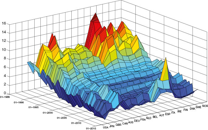
Long-term interest rates 1989–2013.
Behavior of long-term nominal interest rates on 10 years government bonds for the countries in our sample. The sample runs from 1989 to 2013.
This evidence is in line with the hypothesis that countries might be subject to the same shocks causing a co-movement in interest rates. To verify the importance of common factors, we test for the presence of cross-sectional dependence in long-term interest rates and the macroeconomic variables of interest using Pesaran’s (2004)CD test. For a panel of N countries, the test statistic is constructed from the combinations of estimated correlation coefficients. Under the null of cross-sectional independence the statistic is distributed as a standard Normal. For all the variables in our sample we find strong evidence of cross-sectional dependence (Table 2).[11]
Cross sectional dependence test.
| Variable | CD-test | p-Value | Corr | Abs(corr) |
|---|---|---|---|---|
| Long-term int rates | 75.38 | 0 | 0.92 | 0.92 |
| Exp int rates – short | 73.97 | 0 | 0.90 | 0.90 |
| Exp inflation | 46.75 | 0 | 0.57 | 0.57 |
| Exp growth | 39.91 | 0 | 0.49 | 0.50 |
| Exp def/GDP(–1) | 45.5 | 0 | 0.56 | 0.58 |
| Exp debt/GDP(–1) | 26.08 | 0 | 0.32 | 0.41 |
Cross sectional correlation test. Under the null hypothesis of cross-section independence the statistic CDN(0, 1). The table shows the value of the test statistic, the p-value associated to the test and the value and absolute value of the estimated cross-sectional correlation.
We also conducted standard stationarity tests (Table 3). We first implement the Pesaran’s (2007) test for panel unit root and we find indication that almost all the variables can be treated as stationary. There is mixed evidence with respect to the fiscal variables, particularly the public debt. We therefore implement the Moon and Perron’s test (2004) which accounts for multifactor structure, which gives evidence of stationarity for all the variables.[12] We thus conclude that all the variables in our panel can be treated as stationary.
Panel unit root tests.
| CIPS | 0 lag p-Value | CIPS | 1 lag p-Value | CIPS | 2 lag p-Value | MP | p-Value | |
|---|---|---|---|---|---|---|---|---|
| Long-term int rates | –6.07 | 0.00 | –2.41 | 0.01 | –2.05 | 0.02 | –15.49 | 0.00 |
| Int rate – short | –6.51 | 0.00 | –5.73 | 0.00 | –4.96 | 0.00 | –9.27 | 0.00 |
| Inflation | –6.87 | 0.00 | –5.25 | 0.00 | –4.88 | 0.02 | –21.79 | 0.00 |
| Gdp growth | –7.12 | 0.00 | –4.43 | 0.00 | –4.57 | 0.00 | –34.45 | 0.00 |
| Def/GDP(–1) | –1.88 | 0.03 | –1.81 | 0.04 | –1.45 | 0.07 | –21.29 | 0.00 |
| Debt/GDP(–1) | 1.06 | 0.86 | 1.75 | 0.96 | 2.28 | 0.99 | –6.69 | 0.00 |
CIPS is the t-test for unit roots in heterogeneous panels with cross-section dependence, proposed by Pesaran (2007). The lag refers to the order of the ADF regression. Null hypothesis assumes that all series are non-stationary. MP is the Moon and Perron (2004) panel unit root test based on two extracted factors from the variable. The lag order is selected automatically. Null hypothesis assumes all series are non-stationary.
4 Econometric specification and estimation strategy
In this section we describe the FAP technique and discuss its properties and estimation procedure. We derive the estimating equation starting from a data generating process in which a set of global unobservable factors affect both interest rates and macroeconomic variables. This feature generates the pattern of cross-sectional dependence observed in the data (see Section 3). In the next section we discuss the econometric model and show – as in Giannone and Lenza (2008) – that standard estimation techniques are likely to yield biased estimates whenever the effects of global factors are truly heterogeneous across countries. In Section 4.2 we discuss the estimation of the unobserved factors and refer the reader to Section 9, Technical Appendix A for more details.
4.1 The econometric model
Let rit and xit be, respectively the long-term interest rate and a set of observable variables, with (i=1, …, N; t=1, …, T). When looking for the determinants of interest rates the natural starting point is a linear model of the type:
where the country intercepts αi capture time invariant heterogeneity across countries. This is the equation estimated for example by Reinhart and Sack (2000) in a panel of 20 OECD countries. The estimates of the β coefficients are however unlikely to be informative of the effect of xit on rit if these are influenced by a set of unobserved global factors. This is the case for open and integrated economies where there exist common sources of fluctuations – such as common business cycle, common monetary policy. A common shock would in fact jointly determine the reaction of monetary and fiscal authorities across countries and hence the level of interest rates. Following Giannone and Lenza (2008) we therefore assume a factor structure of the type:
in which observable quantities {rit, xit} are a function of a set of q unobservable global factors
Given this data generating process, an accurate estimate of the effect of macroeconomic and fiscal policy variables on interest rates should be based on the idiosyncratic components only:
Equation (3) cannot be estimated because the idiosyncratic components
By taking explicitly into account the global factors
When the data generating process is represented by the system in (2), we can obtain unbiased estimates of the coefficients β only if we allow the factors to have heterogeneous impact across countries (δki≠δkj). This aspect has been often ignored in previous studies. In fact, when tackling the issue of common unobserved factors the literature has mainly pursued different paths. The first approach (Chinn and Frankel 2007) consists of finding an a priori observable variable (or a subset of variables) which might affect contemporaneously the interest rates across countries, and introduce it directly in the panel:
where the variable (zt) is the vector (or matrix) of identified common factors. Alternatively, unobserved factors have been accounted for by introducing time effects. This would lead to the estimation of the following model (Ardagna, Caselli, and Lane 2007):
This is equivalent to assuming that in each time period there is a common shock which affects homogeneously countries’ interest rates.
Differently from the FAP specification in (4), equations (5) and (6) impose homogeneous effects of the global factors, represented either by the common regressors zt or by the time effects τt. If however the unobserved factors have truly an heterogeneous effect across countries, then the country specific components will become part of the error terms of (5) and (6). Therefore, if the factors are correlated with the observable variables- as implied by (2) – equations (5) and (6) will suffer from endogeneity and produce biased estimates.
4.2 Estimation strategy
To obtain consistent estimates of the sets of unobservable factors we follow Giannone and Lenza (2008) and use principal components. This is a general procedure that can be applied whenever in a linear regression the variables have a factor structure. It consists of taking the entire set of dependent and independent variables for all the N cross sections and, after stacking them together in a single matrix, apply principal components.
Hence to estimate the unobserved factors of equation (4), we collect all the variables {rit, xit}i=1, …, N;t=1, …, T in a matrix Wr:
If the elements
The first two eigenvectors explain 69 percent of the panel variance with the third one contributing for less than 10 percent (see Table 4).
Principal component analysis.
| Principal component | |||||
|---|---|---|---|---|---|
| 1st | 2nd | 3rd | 4th | 5th | |
| Marginal | 0.533 | 0.157 | 0.082 | 0.048 | 0.031 |
| Cumulative | 0.533 | 0.690 | 0.772 | 0.820 | 0.850 |
The table reports the marginal and cumulative proportions of the explained variance by the first 5 principal components. The principal components are extracted from the matrix Wr – see Appendix A for details.
Following Giannone and Lenza (2008), we therefore take into consideration only the first two factors. Using these two estimated vectors we can rewrite equation (4) as:
Notice that, while we allow the response to the common factors (δik) to vary across country, we impose the coefficients β to be common to keep the results consistent with those obtained in previous studies. The economic interpretation of the estimated factors
Although having estimated elements in the regression introduces a further source of uncertainty, which normally requires to bootstrap the standard errors, we rely on the result by Giannone and Lenza (2008), Bai (2004) and Bai and Ng (2006) who show that with a relatively large number of countries there is no generated regressor problem.[14] However, we also perform a robustness check estimating the FAP with bootstrap standard errors as in Gonçalves and Perron (2013).[15]
The FAP is however not the only methodology proposed in the literature. Other types of estimator developed to tackle the issue of common unobservable factors and cross-sectional dependence are Pesaran’s (2006) Common Correlated Effect (CCE), and Bai’s (2009) Interactive Fixed Effects (IFE) and Greenaway-McGrevy, Han, and Sul (2012) estimator. In Technical Appendix B we show that our main results are preserved if we employ these alternative estimation techniques.[16]
5 Estimation results
5.1 Baseline model
In this section we present the results from the estimation of equation (7). The results are reported in Table 5. To control for possible structural breaks in the coefficients as a result of the crisis, we report in the first three columns the results excluding the observations before the year 2008, and in the last three columns the results including the latest sample. In the table, columns 1, 2, 4 and 5 use standard panel techniques, while columns 3 and 6 presents the results of the FAP estimation. In particular, we first estimate equation (7) using only country fixed effects αi (columns-FE), then we include also time fixed effects τt (columns-2FE) and finally we include both fixed effects and estimated factors (columns-FAP).[17] At the bottom of each table we include, as a further specification test, the value of the CSD statistic, which is Pesaran’s (2006) test for cross-sectional dependence[18] applied to the residuals of the estimated equation.
Baseline estimation – long-term interest rates.
| Variables | Before 2008 | All sample | ||||
|---|---|---|---|---|---|---|
| (1) | (2) | (3) | (4) | (5) | (6) | |
| FE | 2FE | FAP | FE | 2FE | FAP | |
| Int rate – short | 0.769*** | 0.616*** | 0.357*** | 0.796*** | 0.514*** | 0.331*** |
| [0.035] | [0.060] | [0.040] | [0.022] | [0.058] | [0.042] | |
| Inflation | 0.246*** | 0.195** | 0.083 | 0.044 | 0.079 | 0.069 |
| [0.081] | [0.075] | [0.049] | [0.075] | [0.070] | [0.047] | |
| GDP growth | 0.379*** | 0.087 | 0.105* | 0.007 | –0.228*** | –0.057 |
| [0.102] | [0.070] | [0.057] | [0.089] | [0.062] | [0.092] | |
| Def/GDP(–1) | 0.113*** | 0.054** | 0.016 | 0.076*** | 0.029 | 0.011 |
| [0.017] | [0.018] | [0.013] | [0.018] | [0.019] | [0.013] | |
| Debt/GDP(–1) | 0.019** | 0.006** | 0.008** | 0.012 | 0.005** | 0.011** |
| [0.008] | [0.002] | [0.003] | [0.008] | [0.002] | [0.004] | |
| Observations | 641 | 641 | 641 | 845 | 845 | 845 |
| R2 | 0.855 | 0.959 | 0.981 | 0.834 | 0.935 | 0.963 |
| Number of id | 17 | 17 | 17 | 17 | 17 | 17 |
| CSD | 43.04 | –3.42 | –3.34 | 43.42 | –2.10 | –1.23 |
| Country FE | Yes | Yes | Yes | Yes | Yes | Yes |
| Time FE | No | Yes | Yes | No | Yes | Yes |
| Factors | No | No | Yes | No | No | Yes |
Robust t-statistics in brackets.
***p<0.01, **p<0.05, *p<0.1.
The dependent variable is the long-term nominal interest rate. The independent variables are: expected short term interest rate; expected inflation; expected GDP growth; expected deficit as a share of previous period GDP; expected gross debt as a share of previous period GDP. CSD is the Pesaran’s (2004) statistic to detect cross-sectional dependence; the statistic is distributed as a normal under the null of cross-sectional independence. Column 1 reports the results from the FE; column 2 reports the results from the 2FE and column 3 reports the results from the FAP.
We first discuss the results for the pre-crisis period. Our results show that, when we account for cross-sectional dependence, the impact of domestic variables on long-term interest rates diminishes significantly. We start by looking at the role of fiscal policy. The positive correlation between fiscal variables and long-term interest rates previously found in the literature is not robust when we account for cross-sectional dependence. A standard FE estimator shows that a one percentage point increase in the expected primary deficit to GDP ratio increases interest rates by around 11 basis points, while a 1 percent increase in the expected debt to GDP ratio increases interest rates by around 1.9 basis points (column 1). However, the large value of the CSD statistic (43.04) for the residual, indicates that the regression is misspecified.
Looking at columns 2 and 3 we first notice the importance of accounting for common factors. For both estimators, the CSD statistic falls markedly compared to the FE, but the FAP performs better against the 2FE (–3.42 vs. –3.34). The response of long-term interest rates to domestic fiscal policy diminishes in both cases. When we allow for heterogeneous response to global shocks with the FAP (column 3), the primary deficit becomes statistically insignificant, while the effect of public debt remains significant. As for the magnitude, the effect is smaller than the standard FE estimator (column 1): a 1 percent increase in public debt increases long-term interest rates by around 1 basis point.
The coefficients on the other variables also decrease significantly in magnitude. The coefficient on short-term interest rate decreases when using the FAP, indicating that, accounting for cross-sectional dependence, long-term interest rates are less responsive to domestic monetary policy. The result confirms the findings in the literature that central banks have been progressively losing effectiveness in stirring long-term rates. Giannone, Lenza, and Reichlin (2009), show how in the recent decades long-term interest rates have become more disconnected from country-specific monetary policy stances. The coefficient on GDP growth remains positive but becomes marginally significant. Finally, we find that coefficient on expected inflation becomes insignificant.
We now briefly discuss the results obtained when including the more recent sample. We confirm the importance of accounting for global factors, but the FAP again performs better than the 2FE as shown by the improvement in the CSD statistics (from –2.10 to –1.23). The coefficients on fiscal and monetary policy are almost unaffected, with short-term rate, deficit and debt maintaining similar magnitude and significance. Including the latest crisis changes the significance and signs of the coefficient on GDP growth which becomes negative and ceases to be statistically significant. This shows how growth expectations have started to play a stronger role in assessing fiscal sustainability, with downturns impacting negatively borrowing costs.
5.2 Time variation in the domestic components
In this section we check how the importance of the domestic (idiosyncratic) components has been changing over time. We have shown that, when controlling for global factors, coefficients on domestic variables weaken. We first provide evidence on the changing contributions of the common factors to the total variance in the data. We then show the evolution of the coefficients in the main regression over time and check for possible breaks.
In Figure 2 we compute the variance explained by the first three global factors using a rolling window of 20 periods.
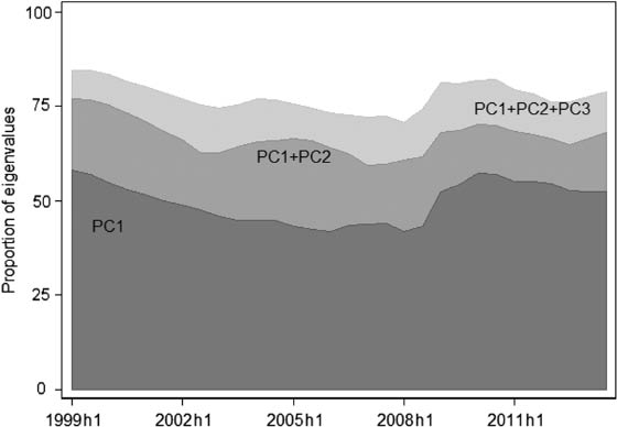
Rolling window estimates – principal components.
The figure report a 20 period rolling window estimate of the proportion of variance explained by the first three principal components.
The figure shows that the share of variance explained by the first three global factors tends to be relatively stable over the sample period, with three principal components explaining between 70 and 80 percent of the variance in the data. We notice that the share of variance explained by the first principal component diminishes over time until the crisis, while the share of variance explained by the second factor increases. After the crisis, the share of variance explained by the first principal component increases up to 60 percent indicating a stronger co-movement of macroeconomic and financial variables in heightened market turmoil, a result found also in different markets (Longstaff et al. 2011; Eichengreen et al. 2012).
We now analyze the time varying effect of domestic fiscal variables.[19] We re-estimate (7) using rolling regressions with a window of 20 periods.[20] We can therefore follow the evolution over time of the coefficients on domestic primary deficit and public debt, and analyze more clearly how the crisis has affected the stability of these coefficients (Figure 3).
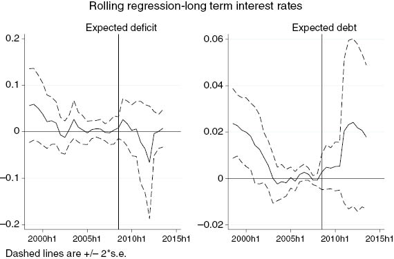
Rolling window estimates – long-term interest rates.
The figures report the rolling window estimates for expected deficit and expected debt obtained from estimating equation (7) with a 20 period rolling window. Dashed lines represent two standard deviation confidence bands.
There is a clear downward trend in the coefficients up until the crisis, indicating weakening influence of domestic variables on interest rates. After the crisis, there is a temporary increase in the importance of domestic fiscal policy. While fiscal deficits do not have any impact through the more recent period, the coefficient on public debt increases but the uncertainties around its estimates also increases due to the large variation observed in debt during this period. We have further analyzed the role played by the crisis by testing for structural breaks in the coefficients interacted with a crisis dummy. The results, available in Technical Appendix B, provide evidence the coefficient on a measure of fiscal sustainability – the “deficit gap” defined as in Faini (2006) – has increased after the crisis. This evidence suggests a possible re-pricing of risk in the aftermath of the global financial crisis [see Sgherri and Zoli (2009) for evidence on the EMU].[21]
5.3 Comparison with existing literature
The results so far indicate that, when we account for heterogeneous response to global shocks: (1) long-term interest rates remain positively related only to public debt; (2) there is mild evidence of increased importance of domestic fiscal policy in the crisis. Our results stand partly in contrast with previous literature. In particular, past studies have found a significant effect of public deficits on long-term interest rates (Ardagna, Caselli, and Lane 2007). We show in this paper that properly accounting for global factors and cross-sectional dependence in the estimation is crucial to understand this result. The omission of such factors leads to overestimating the impact the idiosyncratic component of fiscal policy. Beside lower impact of public deficits, we also find that the effect of public debt on long-term interest rates is smaller compared to previous estimates. Laubach (2009) for instance, finds that a 1 percent increase in public debt to GDP leads to an increase in long-term interest rates by 3–4 basis points. We find that the impact is close to 1 basis point. While we cannot directly compare our estimates to Laubach’s (2009) due to differences in the underlying datasets and specifications used in the estimation, we can refer to Laubach’s analysis (2009) to reconcile our results with economic theory. Within the neoclassical growth model, under the assumption that roughly two-thirds of the increase in public debt is offset by domestic savings, Laubach (2009) shows that a 1 percent increase in public debt to GDP leads to an increase in real interest rates by 2.1 basis points.[22] Recent evidence has however challenged this assumption on the degree crowding-out. Giannone and Lenza (2008), using a Feldstein-Horioka regression, show that less than one-fifth of savings in developed countries are retained for domestic investment. Once a lower degree of crowding-out is assumed, we can reconcile our estimates with theory, and generate effects of public debt on real interest rates in the range of 1 basis point (Table 5, columns 3 and 6).[23]
Our results show that the domestic components of fiscal policy play a smaller role in determining long-term interest rates, once we account for global factors. Previous literature has in fact recognized that, in financially integrated economies, “global fiscal policy” should more prominently explain fluctuations in long-term interest rates compared to domestic fiscal policy. Faini (2006) for example, analyzes the effect of a “global fiscal expansion” for EMU countries. He finds that the effects on interest rates of domestic fiscal policy shocks are rather small compared to those caused by a global fiscal expansion: a change in domestic surplus leads to a 5 basis points reduction of interest rates, while a change in the EMU surplus leads to a 41 basis points decrease in interest rates. Ardagna, Caselli, and Lane (2007) analyze the impact of the world fiscal stance, measured as both the aggregate primary deficit and the aggregate debt, on a sample of OECD countries. They find that, depending on the specification, the world deficit leads to increase in interest rates between 28 and 66 basis points, while world debt increases interest rates between 3 and 21 basis points. Similar results can be found in Claeys, Rosina, and Suriñach (2012).[24] In all cases, the effects are found to be statistically significant and much larger than those of domestic fiscal shocks. Our estimation strategy is well suited to capture the importance of global factors estimated through principal components. The lack of an economic interpretation of what these principal components represent is a possible drawback of the estimation strategy. While a formal analysis of what can constitute these global factors is beyond the scope of this paper, to provide some economic interpretation to these factors, we relate our results to the existing literature and use the FAP estimator to analyze the magnitude and the cross-country differences in the coefficients related to the global factors.
As a first step we plot the principal components against macroeconomic aggregates. We find that the first principal components resemble a measure of aggregate global monetary policy. The second principal component should be a variable which is driven by the same common shocks but not collinear with the monetary stance. As discussed in Technical Appendix A, we find that indeed there is a strong correlation with global fiscal policy stance, a result which is in line with the empirical specifications chosen by the previous literature.[25] To estimate the effects of these global factors we re-estimate equations (7) replacing the estimated factors with their economic interpretation. As discussed in Technical Appendix B we use the average expected primary deficit[26] and the average expected short term rate of the countries in our sample. The estimated coefficients on the global factors are indeed quantitatively important and highly heterogeneous across countries (see Table 6). In line with previous literature, average deficit is by far more important than the idiosyncratic fiscal components. Its average effect is in fact around 20 basis points, which is more than ten times larger than the effect of an increase in idiosyncratic primary deficit. However, contrary to previous literature, the results are highly heterogeneous across countries (F-test rejects hypothesis of homogeneity at less than 1%). Suggestively, coefficients are higher for countries which were less financially integrated at the beginning of the sample or which were characterized by macroeconomic and institutional weaknesses (Figure 4).
Effects of global deficit – long-term interest rates.
| Countries | Global def |
|---|---|
| AUS | 0.186*** |
| (0.063) | |
| AUT | 0.098* |
| (0.050) | |
| BEL | 0.163*** |
| (0.053) | |
| CAN | 0.092 |
| (0.057) | |
| DNK | 0.107* |
| (0.055) | |
| FIN | 0.259*** |
| (0.059) | |
| FRA | 0.134*** |
| (0.050) | |
| DEU | 0.050 |
| (0.051) | |
| IRE | 0.415*** |
| (0.101) | |
| ITA | 0.503*** |
| (0.088) | |
| JPN | 0.132** |
| (0.057) | |
| NLD | 0.075 |
| (0.050) | |
| NOR | 0.065 |
| (0.058) | |
| ESP | 0.466*** |
| (0.092) | |
| SWE | 0.179*** |
| (0.065) | |
| GBR | 0.209*** |
| (0.056) | |
| USA | 0.065 |
| (0.058) | |
| Observations | 845 |
| F test | 3748.81*** |
The table reports the country specific coefficients on the global deficit factor obtained from the estimation of equation (7). The factor is proxied by the average expected budget deficit of the countries in the sample. “F-test” is the value of the F-statistic for the test of equality of coefficients.
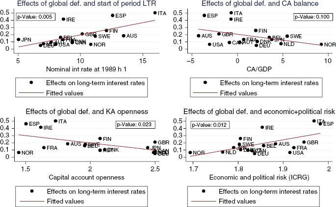
Determinants of the cross-country dispersion of the effects of global deficit.
The figures report the estimated country specific effect of global deficit. They are correlated with measures of initial capital markets integration, current account imbalances and economic and institutional fragility.
6 Discussion and policy implications
The evidence presented so far provides an interesting reading of the recent dynamics of interest rates and useful policy messages. All together our results show that: (1) using an econometric specification which appropriately accounts for cross-sectional correlation, the importance of idiosyncratic (domestic) factors is greatly diminished (Table 5); (2) idiosyncratic factors seem have lost importance over time-with the exception of the crisis period (Figure 3); (3) the effect of global factors is quantitatively more important (Table 6).
Loss of importance of idiosyncratic factors in favor of global ones can be attributed to financial and economic integration and better coordination of macroeconomic policies. Our analysis shows that global factors are highly correlated with global monetary and fiscal policy stance. The compression of long-term interest rates which occurred in OECD countries prior to the crisis could be explained by the fiscal retrenchment which took place among industrialized countries at the beginning of the nineties and the lowering of inflation premia due to a shift to credible inflation targets.
As suggested by the top left plot of Figure 4, convergence has occurred more strongly in countries less financially integrated at the beginning of the sample.[27] However, in these same countries – mostly the peripheral European countries – the compression of long-term interest rates went hand in hand with the build-up of external imbalances. As the coefficients on the second global factor are shown to be related to external vulnerabilities,[28] this can explain why initial convergence of interest rates came to a halt when global conditions suddenly changed.
Overall, we can draw the following policy implications. Since the role of idiosyncratic policies on interest rates is diminished, a first important implication of this result is that countries’ fiscal sustainability should be assessed against variation in global factors (Gonzalez-Rozada and Levy Yeyati 2008). Furthermore, since domestic policies have small direct impact on interest rates, but rather have an indirect impact through global factors, these spillovers can have large effect on countries characterized by external vulnerabilities. Improvement in the underlying fundamentals and better international policy coordination[29] can therefore help countries gain better control of their interest rates.
7 Concluding remarks
In this paper we tackled the issue of identifying the effects of domestic fiscal policy on long-term interest rates for a panel of OECD countries. We use real time data on forecasts to better take into account the forward looking nature of the responses of financial markets. The strong correlation observed across interest rates in different countries justifies the use of an estimator which takes into account the presence of unobservable global factors. We use a FAP, an estimation procedure originally developed by Giannone and Lenza (2008). This methodology allows us to obtain consistent estimates of the parameters and to study the heterogeneity of the cross-country propagation of global shocks. We show that in general two unobserved factors can explain almost 70 percent of the variance in the data. We find these factors to closely track the aggregate monetary policy and the aggregate fiscal policy stances. Our results show that global factors are not only quantitatively relevant determinants of long-term interest rates, but once introduced in the analysis, they also affect the importance of the idiosyncratic components. When using the FAP estimation method, the role of domestic fiscal policy variables is largely reduced: public debt is still significant, but contributes by only 1 basis point.
We show that the importance of the idiosyncratic factors is time-varying. We show that the role of idiosyncratic factors has been declining over time. However, the results point also to an increase in the sensitivity of interest rates to domestic debt after the global crisis. As for the role played by global factors, we find, in line with previous literature, that the effects of a global fiscal expansion are by far quantitatively more important than domestic fiscal policy alone, but that they are also significantly heterogeneous across countries. The magnitude of these effects ranges between 5 and 51 basis points with stronger effects for countries that are characterized by external, economic or institutional fragilities.
Our results provide an interpretation of the recent behavior of interest rates in advanced economies. While during the nineties the general movement towards fiscal consolidation and low monetary policy rates has contributed to low long-term interest rates, during these last years the increase in countries’ budget deficits have reversed this process. These shocks have triggered a heterogeneous increase in borrowing costs with larger effects for those countries which, while benefiting from the capital markets integration, had also accumulated larger imbalances. Countries’ fiscal and macroeconomic policies therefore, affect interest rates not so much directly, but rather indirectly by influencing the magnitude of the spillover effects from global factors. Hence, even if on one hand economic and financial integration and policy coordination reduce the impact of national policies on borrowing costs, on the other hand changes in global conditions expose more vulnerable countries to a sudden reversal of fortunes.
The views expressed in this paper are those of the author(s) and do not necessarily represent the views of the IMF, its Executive Board, or IMF management.
Appendix A: Variables.
| Variable | Description | Source |
|---|---|---|
| r | Long-term Nominal rate | Datastream |
| r(real) | Difference between r and the trend of expected inflation (infl) | Datastream |
| r–rB | (r–rB) – (sw−swB) | Datastream |
| Interest rate spread minus the difference in interest rate swaps over the same maturity | ||
| stnr | One year ahead short-term (3-month) interest rate | OECD |
| rB | One year ahead long-term nominal interest rate of the benchmark country | OECD |
| infl | One year ahead GDP deflator inflation rate (ln(PGDP_t+1/PGDP_t)) | OECD |
| g | One year ahead growth rate of real GDP | OECD |
| pdef | Government lending net of interest payments (NLG+YPEPG) | OECD |
| debt | Gross Government Financial Liabilities (GGFL) | OECD |
| liq | Ratio of government debt over the total government debt of OECD countries | OECD |
| VIX | Chicago Board Options Exchange Market Volatility Index | Datastream |
| def gap | (gbaI*−gbal) with: gbal*=(rltr−g)debt, and gbal=−pde and rltr=ltr-irf, and ltr is the one year ahead forecast for long-term rate | OECD |
Technical Appendix A: Estimation details
The aim of this appendix is to provide more details on the extraction of the factors and present the evidence for their economic interpretation. As mentioned in Section 4.2 we follow Giannone and Lenza (2008) and we estimate the unobserved factors of equation (7) by means of principal components. The principal components are extracted from the variance covariance matrix of Wr, which contains the observable left-hand side and right-hand side variables of equation (7):
where r is the (T×N) matrix of long-term interest rates, stnr the matrix of expected short-term rates, infl is the matrix of expected inflation rates, g that of expected real GDP growth rates and pdef and debt those of expected primary deficits and public debts, respectively. As mentioned in the text, interest rates “r” are measured after the release of the forecasts in order to avoid reverse causality from interest rates to macroeconomic and fiscal variables. Now, because factors extracted with PC can be considered exogenous to the variables included in the W matrix, the parameters β in equation (4) correctly identifies the causal effect of idiosyncratic macroeconomic and fiscal variables on the idiosyncratic components of interest rates.
A first important decision in our analysis is the determination of the number of factors to include in the regression. In the empirical literature on factor models, the determination of the number of factors has been a subject of intense research. For example, Forni and Reichlin (1998) propose a rule of thumb according to which one should retain the number of principal components that explains more than a certain fraction of the variance, while Bai and Ng (2006) present a formal test based on information criteria. In our case, as shown in Table 4 in the text, the first two components extracted from Wr explain about 68 percent of the total variance, with third factor contributing for about 7.8 percent. Following the rule of thumb proposed by Giannone and Lenza (2008) we decide therefore to include two factors in the estimating equation.
A second important point is the economic interpretation of the common factors. To find it we follow economic intuition. It is plausible to think that in integrated capital markets the global factors driving the interest rates must be related to the global availability of funds. Aggregate supply of savings is in turn affected by the aggregate fiscal stance – which is the “public” component of savings – and by aggregate monetary policy stance, which drives the availability of liquidity in the market. This intuition is well supported by the data. In fact the first two factors extracted from Wr are very much correlated with the average expected short term interest rate and with the average expected primary deficit (Figure 5).[30]

Global factors and their macroeconomic interpretation.
The Figure shows the estimated unobserved factors plotted against their economic interpretation. The top panel shows the first factor plotted against the average expected short-term interest rate of the countries in the sample. The lower panel shows the second factor plotted against the average expected deficit of the countries in the sample.
To give quantitative support to our interpretation, we then try to regress our estimated factors on the average short term rate and on the average deficit, respectively. Table 7 reports the results of this exercise. In both cases the constant term is close to zero and never significant, while the coefficient on the estimated factor is close to one for the short-term rate and close to 0.7 for the deficit. In both cases the coefficients are strongly significant. The R2 also indicates a good fit. Given that the extracted factors are standardized, we also standardize the short term interest rates and the deficits before computing the averages across countries.
Interpretation of the global factors – long-term interest rates.
| Variables | (1) 1st PC | (2) 2nd PC |
|---|---|---|
| Average int rate | 0.984*** | |
| (0.0261) | ||
| Average def | 0.670*** | |
| (0.107) | ||
| Constant | 6.56e–09 | 1.92e–09 |
| (0.0258) | (0.106) | |
| Observations | 50 | 50 |
| R2 | 0.967 | 0.449 |
Standard errors in parentheses.
***p<0.01, **p<0.05, *p<0.1.
In column 1, the dependent variable is the first principal component extracted from Wr while the independent variable is the average expected short term interest rate of the countries in the sample. In column 2, the dependent variable is the second principal component extracted from Wr while the independent variable is the average expected deficit of the countries in the sample.
The extraction of the factors is done in an analogous manner for the specifications for the real interest rate and the sovereign spreads (Figure 5 and Tables 7 and 8).
Baseline estimation – real interest rates and sovereign spreads.
| Variables | (1) Real rates | (2) Spreads |
|---|---|---|
| Int rate – short | 0.287*** | |
| [0.040] | ||
| Inflation | –0.452*** | |
| [0.072] | ||
| Int rate – benchmark | 0.169 | |
| [0.156] | ||
| Liquidity | –0.137** | |
| [0.056] | ||
| GDP Growth | –0.042 | –0.061 |
| [0.101] | [0.044] | |
| Def/GDP(–1) | 0.035** | 0.011 |
| [0.014] | [0.007] | |
| Debt/GDP(–1) | 0.012** | 0.015*** |
| [0.005] | [0.005] | |
| D(EMU) | –1.166** | |
| [0.557] | ||
| Observations | 845 | 476 |
| R2 | 0.926 | 0.565 |
| Number of id | 17 | 15 |
| CSD | –1.89 | –0.98 |
| Country FE | Yes | Yes |
| Time FE | Yes | Yes |
| Factors | Yes | Yes |
Robust t-statistics in brackets.
***p<0.01, **p<0.05, *p<0.1.
The table shows the results of estimating equation (7) using the real interest rate (column 1) and sovereign spreads (column 2) as dependent variables. The real interest rate is computed as the long-term interest rate minus the trend component of expected inflation which is computed applying a Kalman filter to the expected inflation. Spreads are computed with respect to the German long-term interest rate for EMU countries and to the US long-term interest rate for the other countries. They are adjusted for the exchange rate risk following Codogno, Favero, and Missale (2003). The independent variables from top to bottom are: expected short term interest rate; expected inflation; the expected long-term interest rate of the benchmark country (Germany for EMU countries and US for the rest); liquidity, measured as the ratio between the stock of sovereign debt and the total debt of OECD countries; expected GDP growth; expected deficit as a share of previous period GDP; expected gross debt as share of previous period GDP; a dummy variable for the introduction of the EURO. CSD is the Pesaran’s (2004) statistic to detect cross-sectional dependence; the statistic is distributed as a normal under the null of cross-sectional independence.
In particular, for the specification with the real interest rates, we extract the factors from the variance covariance matrix of Wreal, which contains:
where r(real) is our measure of long-term real interest rate. When we estimate the specification for the sovereign spreads, instead, we extract the factors from a matrix Wspreads which is constructed as:
The long-term interest rates r have been replaced by the sovereign spreads and the expected long-term interest rate of the benchmark country rB. The VIX is the Chicago Board Options Exchange Market Volatility Index. Additionally we introduced a measure of liquidity [the ratio of government debt over the total debt of the OECD countries as in Gomez-Puig (2006)], which is usually included as a control in an equation for the spreads.
In terms of the importance of the global factors, in the first case the results are very similar to those for the long-term nominal rate: two factors explain more than two thirds of the panel variance and are interpretable as global fiscal and monetary policy stance as they track very closely the average expected deficit and the average expected short-term interest rate. In the second case, a third factor becomes relevant and it tracks very closely the dynamics of the VIX index. We interpret this factor as the “global risk aversion” factor [as in Sgherri and Zoli (2009)].[31]
Technical Appendix B: Robustness checks
Results from different specifications
In this section we report the results from using different left-hand side variables. We first measure the impact of fiscal policy on the real interest rate. Since the ex-ante real long term yield is unobservable, as in Ardagna, Caselli, and Lane (2007) we construct it from the data. Since the Outlook provides forecast only for inflation in period t+1, we proxy inflation expectations in t+10 with the “trend inflation” calculated with the help of a Kalman Filter applied recursively on the series of inflation expectations for the year t+1. As a second exercise, we measure the impact of fiscal policy on the yield spreads measured as the difference between the ten years yield and the yield on a risk-free asset of the same maturity (r–rB).[32] To correct for the presence of exchange rate risk, we follow Codogno, Favero, and Missale (2003) and before computing the spreads we subtract from the long-term interest rates the different on the interest rate swaps of the same maturity denominated in different currencies.[33] However, because of the availability of data on interest rate swaps, the sample covers the period 1997–2013.
Before estimating the FAP equations for the real interest rate and the spreads equation we have to re-estimate the global factors for each of these two specifications. In the first case the results are very similar to the ones obtained for the equation for long-term nominal rates: two global factors account for more than two thirds of the variance and they can be interpreted as the global monetary and the global fiscal policy stances. For the spreads equation, instead, the relevant factors seem to be three: besides global monetary and fiscal policy stances a third factor which mimics global risk aversion is very relevant (see Technical Appendix A).[34] The results are reported in Table 8.
The effect of domestic deficits on the real interest rate is still statistically significant and the value of the coefficient is of 3 basis points. As for the level of public debt, instead its effect stays significant and it is about one and a half basis points. The expected short term interest rate is positive and significant, with a magnitude comparable to what found when examining the effect on long-term nominal rates (Table 5). The coefficient on GDP growth is negatively signed but not statistically significant. Finally, we find a negative relation with the expected inflation. This is a direct consequence of allowing for an open economy setting. In open economies, in fact, nominal rates will rise less than one-for-one with inflation because of a substitution from money to bonds, thus higher expected inflation reduces ex-ante real interest rates [the “Mundell-effect,” Mundell (1963)] (Table 8 column 1).
When estimating the equation for sovereign yield spreads, we include also a measure of liquidity (the ratio of the stock of public debt over the total debt of OECD countries)[35] and a dummy variable for the introduction of the Euro to control for the flattening of sovereign spreads after the introduction of the single currency [as in Schuknecht, von Hagen, and Wolswijk (2011)]. The fiscal variables turn out to be correctly signed but only the coefficient on public debt is statistically significant. Its effect is about one and a half basis point. The sign and significance of the EMU dummy variable are consistent with the empirical evidence of a strong convergence of sovereign spreads in the Euro area after the introduction of the single currency. The results differ from the ones using the nominal rates but the two cannot be directly compared since the estimation is performed over different sample periods (Table 8 column 2).
Robustness checks
In this section we present the results of a series of other robustness checks. As a first check we re-estimated equation (7) replacing the factors estimated from principal components with what we found to be their economic interpretation. That is, we replicate the results of the third column in Table 5 but instead of the estimated factors we use the average expected deficit and the average expected short term interest rate. The results (column 2, Table 9) are remarkably similar to those obtained with the estimated factors (column 1, Table 9). The test statistic of cross-sectional dependence on the residuals is also remarkably similar. We interpret these results as a further validation of our interpretation for the estimated factors.
Factors’ interpretation – long-term interest rates.
| Variables | (1) FAP | (2) Macro F |
|---|---|---|
| Int rate – short | 0.331*** | 0.381*** |
| [0.042] | [0.044] | |
| Inflation | 0.069 | 0.054 |
| [0.047] | [0.062] | |
| GDP growth | –0.057 | –0.099 |
| [0.092] | [0.107] | |
| Def/GDP(–1) | 0.011 | 0.008 |
| [0.013] | [0.013] | |
| Debt/GDP(–1) | 0.011** | 0.011*** |
| [0.004] | [0.003] | |
| Observations | 845 | 845 |
| R2 | 0.963 | 0.957 |
| Number of id | 17 | 17 |
| CSD | –1.23 | –1.01 |
| Country FE | Yes | Yes |
| Time FE | Yes | Yes |
| Factors | Yes | Yes |
Robust t-statistics in brackets.
***p<0.01, **p<0.05, *p<0.1.
The dependent variable is the long-term nominal interest rate. The independent variables from top to bottom are: expected short term interest rate; expected short-term interest rate; expected Inflation; expected GDP growth; expected deficit as a share of previous period GDP; expected gross debt as a share of previous period GDP. Column 1 repeats the results from the baseline specification. In column 2 the common factors have been replaced by their interpretation: average short term interest rate and average deficit. CSD is the Pesaran’s (2004) statistic to detect cross-sectional dependence; the statistic is distributed as a normal under the null of cross-sectional independence.
The second robustness check we perform is a cross-validation. We check whether the results from our baseline specifications are confirmed if we exclude from the estimation one country at a time. We notice that the results are remarkably stable, with the expected short-term interest rate and the debt to GDP ratio being consistently significant and of similar magnitude. Expected inflation becomes marginally significant when Finland and Spain are excluded from the sample (Table 10).
Cross validation – long-term interest rates.
| Variables | (1) All sample | (2) No AUS | (3) No AUT | (4) No BEL | (5) No CAN | (6) No DNK | (7) No FIN | (8) No FRA | (9) No DEU |
|---|---|---|---|---|---|---|---|---|---|
| Int rate – short | 0.331*** | 0.299*** | 0.329*** | 0.332*** | 0.344*** | 0.357*** | 0.323*** | 0.331*** | 0.331*** |
| [0.042] | [0.035] | [0.044] | [0.044] | [0.043] | [0.035] | [0.043] | [0.043] | [0.044] | |
| Inflation | 0.069 | 0.062 | 0.071 | 0.071 | 0.080 | 0.054 | 0.091* | 0.069 | 0.071 |
| [0.047] | [0.051] | [0.048] | [0.047] | [0.048] | [0.050] | [0.043] | [0.048] | [0.049] | |
| GDP growth | –0.057 | –0.050 | –0.054 | –0.064 | –0.066 | –0.045 | –0.105 | –0.060 | –0.047 |
| [0.092] | [0.092] | [0.095] | [0.094] | [0.098] | [0.094] | [0.090] | [0.095] | [0.093] | |
| Def/GDP(–1) | 0.011 | 0.011 | 0.011 | 0.011 | 0.016 | 0.012 | 0.011 | 0.011 | 0.011 |
| [0.013] | [0.013] | [0.013] | [0.013] | [0.012] | [0.013] | [0.014] | [0.013] | [0.013] | |
| Debt/GDP(–1) | 0.011** | 0.012** | 0.011** | 0.011** | 0.011** | 0.011** | 0.011** | 0.011** | 0.011** |
| [0.004] | [0.004] | [0.004] | [0.004] | [0.005] | [0.004] | [0.004] | [0.004] | [0.004] | |
| Observations | 845 | 795 | 796 | 795 | 795 | 795 | 795 | 795 | 795 |
| R2 | 0.963 | 0.963 | 0.962 | 0.962 | 0.962 | 0.962 | 0.960 | 0.961 | 0.962 |
| CSD | 17 | 16 | 16 | 16 | 16 | 16 | 16 | 16 | 16 |
| Number of id | –1.23 | –0.75 | –1.93 | –1.11 | –1.25 | –1.38 | –1.13 | –2.03 | –1.81 |
| Country FE | Yes | Yes | Yes | Yes | Yes | Yes | Yes | Yes | Yes |
| Time FE | Yes | Yes | Yes | Yes | Yes | Yes | Yes | Yes | Yes |
| Factors | Yes | Yes | Yes | Yes | Yes | Yes | Yes | Yes | Yes |
| Variables | (10) No IRE | (11) No ITA | (12) No JPN | (13) No NLD | (14) No NOR | (15) No ESP | (16) No SWE | (17) No GBR | (18) No USA |
| Int rate – short | 0.321*** | 0.330*** | 0.330*** | 0.327*** | 0.330*** | 0.338*** | 0.339*** | 0.326*** | 0.337*** |
| [0.042] | [0.043] | [0.045] | [0.044] | [0.048] | [0.041] | [0.043] | [0.046] | [0.046] | |
| Inflation | 0.072 | 0.062 | 0.058 | 0.070 | 0.055 | 0.094** | 0.043 | 0.082 | 0.071 |
| [0.051] | [0.046] | [0.049] | [0.050] | [0.055] | [0.038] | [0.048] | [0.048] | [0.048] | |
| GDP growth | –0.070 | –0.027 | –0.075 | –0.063 | –0.066 | 0.014 | –0.054 | –0.075 | –0.065 |
| [0.111] | [0.096] | [0.096] | [0.098] | [0.103] | [0.064] | [0.096] | [0.095] | [0.099] | |
| Def/GDP(–1) | 0.007 | 0.012 | 0.017 | 0.011 | –0.000 | 0.017 | 0.005 | 0.009 | 0.014 |
| [0.012] | [0.014] | [0.014] | [0.013] | [0.022] | [0.011] | [0.013] | [0.014] | [0.014] | |
| Debt/GDP(–1) | 0.008** | 0.012** | 0.014** | 0.011** | 0.011** | 0.010** | 0.009* | 0.011** | 0.011** |
| [0.003] | [0.004] | [0.005] | [0.004] | [0.005] | [0.004] | [0.004] | [0.004] | [0.004] | |
| Observations | 795 | 799 | 795 | 795 | 795 | 795 | 795 | 795 | 795 |
| R2 | 0.972 | 0.964 | 0.964 | 0.962 | 0.962 | 0.965 | 0.961 | 0.962 | 0.963 |
| CSD | 16 | 16 | 16 | 16 | 16 | 16 | 16 | 16 | 16 |
| Number of id | –2.42 | –1.69 | –1.44 | –1.86 | –1.13 | –2.09 | –0.76 | –1.29 | –1.15 |
| Country FE | Yes | Yes | Yes | Yes | Yes | Yes | Yes | Yes | Yes |
| Time FE | Yes | Yes | Yes | Yes | Yes | Yes | Yes | Yes | Yes |
| Factors | Yes | Yes | Yes | Yes | Yes | Yes | Yes | Yes | Yes |
Robust t-statistics in brackets; ***p<0.01, **p<0.05, *p<0.1.
In this exercise we repeat the estimation of the FAP for the baseline model (equation 7) excluding one country at the time.
The dependent variable is the long-term nominal interest rate. The results are obtained with the FAP.
As a third robustness check we re-estimate our baseline equation using different techniques: Pesaran’s (2006) Common Correlated Effect (CCE) and Mean Group (MG) estimators; Bai’s (2009) Interactive Fixed Effects (IFE) estimator. We also re-estimate the FAP applying the bootstrap method proposed by Gonçalves and Perron (2013) to correct for the fact that our cross-section dimension (N=17) is smaller than the time-series dimension (T=48), thus correcting for sampling uncertainty around the extracted factors. The (CCE) estimator consists of introducing cross-sectional averages of the dependent and the independent variables in the equation. Since cross-country aggregates average out idiosyncratic components, for large cross-sectional dimensions they tend to approximate the common factors. Contrary to the FAP this method does not provide us with a direct estimate of the unobserved factors, which is something we are interested in. Bai (2009) instead, has recently suggested the use of an estimator called Interactive Fixed Effects (IFE) which combines standard OLS and principal components, and calculates the common factors directly from the residual. Results are reported in Table 11.
Baseline estimation – alternative estimation techniques: CCE-MG-IFE-GP.
| Variables | (1) MG | (2) CCE | (3) IFE | (4) GP | |||||
|---|---|---|---|---|---|---|---|---|---|
| Int rate – short | 0.300*** | 0.483*** | 0.324** | 0.333*** | |||||
| [6.598] | [14.006] | [2.476] | [4.691] | ||||||
| Inflation | 0.103** | 0.076* | 0.058 | 0.062 | |||||
| [2.590] | [1.722] | [0.185] | [0.661] | ||||||
| GDP growth | –0.030 | –0.096 | 0.019 | –0.049 | |||||
| [–0.327] | [–1.570] | [0.078] | [–0.516] | ||||||
| Def/GDP(–1) | 0.020 | 0.107*** | 0.005 | 0.012 | |||||
| [1.118] | [4.802] | [0.286] | [0.709] | ||||||
| Debt/GDP(–1) | 0.003 | 0.019*** | 0.007*** | 0.011*** | |||||
| [0.550] | [3.438] | [19.191] | [3.073] | ||||||
| Observations | 845 | 845 | 845 | 845 | |||||
| Number of id | 17 | 17 | 17 | 17 | |||||
Robust t-statistics in brackets.
***p<0.01, **p<0.05, *p<0.1.
Columns 1 reports the results from Pesaran’s MG estimator; column 2 reports the results obtained using Pesaran’s (2006) CCE estimator; column 3 reports the results obtained using Bai’s (2009) Interacted Fixed Effects estimator; column 4 reports the results obtained using the Gonçalves and Perron (2013) estimator. The dependent variable is the long-term interest rate.
When using the MG and CCE estimators both the coefficients of debt and deficit are not statistically significant, while the coefficient on inflation becomes significant. Instead, when we use Bai’s (2009) Interacted Fixed Effects method or Gonçalves and Perron (2013) estimator, our results on the effects of fiscal variables are consistent with what obtained using the FAP.
The existing literature (see Sgherri and Zoli (2009) among others) have pointed out that countries’ fiscal variables might have stronger impact in determining interest rates during crisis periods. We have found some mild evidence that this might be the case when performing the estimates with rolling windows (see Section 5.2). Here we implement a more formal test by re-estimating equation (7) and checking for structural breaks in the coefficients. In the first three columns of Table 12 we interact the coefficients of deficit and debt with two dummy variables: one which takes value 1 before 2007 and another which takes value 1 from that moment onwards. The results show no evidence that the coefficient on the debt to GDP ratio might have increased during the crisis period. The last column of Table 11 includes a new variable, the deficit gap which is computed as in Faini (2006)[36] to check whether the structural break could be pertinent to variables which are more directly linked to expected fiscal sustainability. The results in column 4 of Table 12 support this hypothesis as the value of the coefficient on the deficit gap more than doubles after 2007.[37]
Non-linearity with crises – long-term interest rates.
| Variables | (1) Def Break | (2) Debt Break | (3) Def, debt Break | (4) Def gap Break |
|---|---|---|---|---|
| Int rate – short | 0.331*** | 0.331*** | 0.331*** | 0.365*** |
| [0.042] | [0.043] | [0.043] | [0.044] | |
| Inflation | 0.067 | 0.070 | 0.068 | 0.153*** |
| [0.046] | [0.048] | [0.047] | [0.051] | |
| GDP growth | –0.057 | –0.057 | –0.058 | 0.058 |
| [0.093] | [0.092] | [0.092] | [0.083] | |
| Debt/GDP(–1) | 0.011** | 0.011** | ||
| [0.004] | [0.005] | |||
| Def/GDP(–1) | 0.011 | |||
| [0.013] | ||||
| Time>2007*(Debt/GDP(–1)) | 0.011* | 0.011* | ||
| [0.005] | [0.006] | |||
| Time<2007*(Debt/GDP(–1)) | 0.011*** | 0.011*** | ||
| [0.004] | [0.004] | |||
| Time>2007*(Def/GDP(–1)) | 0.013 | 0.013 | ||
| [0.017] | [0.017] | |||
| Time<2007*(Def/GDP(–1)) | 0.008 | 0.008 | ||
| [0.016] | [0.016] | |||
| Time>2007*(Def Gap) | 0.106* | |||
| [0.059] | ||||
| Time<2007*(Def Gap) | 0.054** | |||
| [0.020] | ||||
| Observations | 845 | 845 | 845 | 845 |
| R2 | 0.963 | 0.963 | 0.963 | 0.963 |
| Number of id | 17 | 17 | 17 | 17 |
| CSD | –1.24 | –1.26 | –1.25 | –1.23 |
Robust t-statistics in brackets.
***p<0.01, **p<0.05, *p<0.1.
The dependent variable is the long-term interest rate. The independent variables from top to bottom are: expected short term interest rate; expected short-term interest rate; expected inflation; expected GDP growth; expected deficit as a share of previous period GDP; expected gross debt as a share of previous period GDP. In columns 1, 2 and 3 we test a specification with a spline on the fiscal variables according to weather or not they are measured after the second half of 2008. In columns 4 we test a spline on the deficit gap (as defined in Appendix B) according to weather or not they are measured after the second half of 2008. CSD is the Pesaran’s (2004) statistic to detect cross-sectional dependence; the statistic is distributed as a normal under the null of cross-sectional independence. All results are obtained using the FAP.
We also check whether, as suggested by Ardagna, Caselli, and Lane (2007), the effect of public debt is non-linear carrying stronger effects after a given level (see Table 13). We re-estimate equation (7) including first a quadratic term for the debt to GDP ratio and then including a spline for the coefficient on public debt at 50 percent and 75 percent of GDP. Our results show that the coefficient on the debt is statistically different when it is higher than 75 percent of GDP. However the difference in the effect is of about 0.3 basis points only and therefore not economically significant.
Non-linearity with public debt – long-term interest rates.
| Variables | (1) Squared term | (2) Spline 50% | (3) Spline 75% |
|---|---|---|---|
| Int rate – short | 0.333*** | 0.331*** | 0.336*** |
| [0.042] | [0.042] | [0.040] | |
| GDP growth | –0.057 | –0.055 | –0.054 |
| [0.092] | [0.091] | [0.091] | |
| Inflation | 0.073 | 0.071 | 0.066 |
| [0.048] | [0.047] | [0.048] | |
| Def/GDP(–1) | 0.011 | 0.011 | 0.012 |
| [0.013] | [0.013] | [0.012] | |
| Debt/GDP(–1) | 0.014 | ||
| [0.008] | |||
| (Debt/(GDP(–1))2) | –0.000 | ||
| [0.000] | |||
| Debt/(GDP(–1)<50% | 0.010* | ||
| [0.005] | |||
| Debt/(GDP(–1)>50% | 0.010** | ||
| [0.004] | |||
| Debt/(GDP(–1)<75% | 0.007* | ||
| [0.004] | |||
| Debt/(GDP(–1)>75% | 0.010** | ||
| [0.004] | |||
| Observations | 845 | 845 | 845 |
| R2 | 0.963 | 0.963 | 0.963 |
| Number of id | 17 | 17 | 17 |
| CSD | –1.31 | –1.34 | –1.11 |
| CIPS-error | 0.00 | 0.00 | 0.00 |
| Test debt | 0.47 | 0.06 | |
Robust t-statistics in brackets.
***p<0.01, **p<0.05, *p<0.1.
The dependent variable is the long-term nominal interest rate. The independent variables are: expected short term interest rate; expected inflation; expected GDP growth; expected deficit as a share of previous period GDP; expected gross debt as a share of previous period GDP. We test different non linearities with respect to public debt: in column 1 we introduced debt to GDP ratio squared; in column 3 and 4 we splined the debt to GDP ratio according to whether it is larger or smaller than 50 percent and 75 percent. CSD is the Pesaran’s (2004) statistic to detect cross-sectional dependence; the statistic is distributed as a normal under the null of cross-sectional independence. All results are obtained using the FAP. “Test debt” reports the p-value of the t-test on the coefficients of the spline for the debt to GDP ratio.
We also checked the correlation between the factors extracted through PCA and their economic interpretation (see Technical Appendix A).
Finally, in Table 14, we repeated the estimation introducing a lagged dependent variable to control for possible omitted variable due to the persistence in long-term interest rates. Given the large time-series dimension in our panel, the Nickell bias is negligible and we can use traditional within-group estimates (column 1). We also introduced a third factor in the estimation. We also estimate the model using the estimator proposed by Gauibollev at al. (2014) (GSS) which allows for factor structure of the regressors as well as lagged dependent variable as in Greenaway-McGrevy, Han, and Sul (2012) (column 3). The results are robust.
Dynamic model and 3-factors FAP.
| (1) Lagged LTR | (2) 3 Factors | (3) GSS | |
|---|---|---|---|
| Lagged LTR | 0.451*** | 0.137*** | |
| [0.024] | [0.048] | ||
| Int rate – short | 0.162*** | 0.153*** | 0.132*** |
| [0.029] | [0.034] | [0.031] | |
| Inflation | 0.012 | 0.027 | 0.058* |
| [0.035] | [0.029] | [0.038] | |
| GDP growth | –0.037 | –0.065 | –0.108** |
| [0.071] | [0.074] | [0.065] | |
| Def/GDP(–1) | 0.013 | 0.012 | –0.009 |
| [0.010] | [0.011] | [0.013] | |
| Debt/GDP(–1) | 0.006* | 0.005 | 0.009*** |
| [0.003] | [0.005] | [0.004] | |
| Observations | 828 | 811 | 811 |
| R2 | 0.969 | 0.969 | 0.969 |
| Number of id | 17 | 17 | 17 |
| CSD | –1.00 | –0.98 | –1.00 |
Robust t-statistics in brackets.
***p<0.01, **p<0.05, *p<0.1.
In columns 1 and 2, the dependent variable is the long-term nominal interest rate. Column 1 performs a dynamic estimation while column 2 adds a third factor to the FAP. Column 3 performs the estimator of Greenaway-McGrevy, Han, and Sul (2012) as discussed in Gaibulloev, Sandler, and Sul (2014).
Finally, we have computed scatter plot in Figure 4 of the paper, by eliminating peripheral European countries (Ireland, Italy and Spain). The results, reported in Figure 6, show that after the removal of peripheral European countries the results remain qualitatively similar although the p-value of the fitted lines increases to non-significant values. Figure 7 reports the results on the rolling regression for the remaining control variables, showing similar decline in the coefficients as in Figure 3 of the paper.
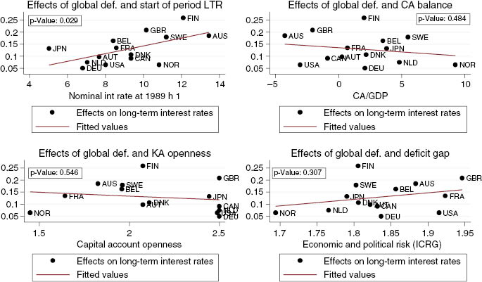
Scatter plots without peripheral Europe.
The figures report the estimated country specific effect of global deficit, excluding peripheral Europe (Ireland, Italy, Spain). They are correlated with measures of initial capital markets integration, current account imbalances and economic and institutional fragility.
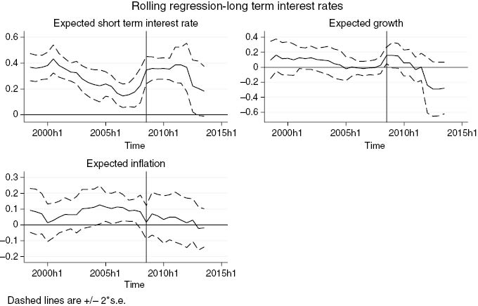
Rolling window estimates – long-term interest rates.
The figures report the rolling window estimates for expected interest rate (short-term) and expected growth and inflation obtained from estimating equation (7) with a 20 period rolling window. Dashed lines represent two standard deviation confidence bands.
We conducted several other robustness checks. We repeated the estimations splitting the sample to consider separately data belonging to the June and to the December issues of the OECD forecasts and obtained similar results. We also repeated the estimation for long-term interest rates checking for the presence of structural breaks after the introduction of the Euro. We used a spline regression where all the regressors entered the equation also interacted with a dummy variable for the introduction of the Euro. We found evidence of a break in the coefficient on the inflation rate, which is positive and significant only for countries and periods not belonging to the EMU. We interpret this result as the “credibility effect” due to the presence of an inflation averse Central Bank.[38]
References
Afonso, Antonio. 2010. “Long-term Government Bond Yields and Economic Forecasts: Evidence for the EU.” Applied Economics Letters, Taylor and Francis Journals 17 (15): 1437–1441.10.1080/13504850903049627Search in Google Scholar
Ardagna, Silvia, Francesco Caselli, and Timothy Lane. 2007. “Fiscal Discipline and the Cost of Public Debt Service: Some Estimates for OECD Countries.” The B.E. Journal of Macroeconomics 7 (1): 1–35.10.3386/w10788Search in Google Scholar
Artis, Michael, and Massimiliano Marcellino. 2001. “Fiscal Forecasting: The Track Record of the IMF, OECD and EC.” Econometrics Journal 4 (1): S20–S36.10.1111/1368-423X.00051Search in Google Scholar
Bai, Jushan. 2004. “Estimating Cross-section Common Stochastic Trends in Nonstationary Panel Data.” Journal of Econometrics 122 (1): 137–183.10.1016/j.jeconom.2003.10.022Search in Google Scholar
Bai, Jushan. 2009. “Panel Data Models With Interactive Fixed Effects.” Econometrica 77 (4): 1229–1279.10.3982/ECTA6135Search in Google Scholar
Bai, Jushan, and Serena Ng. 2006. “Confidence Intervals for Diffusion Index Forecasts with a Large Number of Predictors.” Econometrica 74 (4): 1133–1150.10.1111/j.1468-0262.2006.00696.xSearch in Google Scholar
Beetsma, Roel, and Massimo Giuliodori. 2010. “Fiscal Adjustment to Cyclical Developments in the OECD: An Empirical Analysis Based on Real-time Data.” Oxford Economic Papers 62 (3): 419–441.10.1093/oep/gpp039Search in Google Scholar
Bernoth, Kerstin, Jurgen Von Hagen, and Ludger Schuknecht. 2004. “Sovereign Risk Premia in the European Government Bond.” Working Paper Series 369, European Central Bank.10.2139/ssrn.533129Search in Google Scholar
Canzoneri, Matthew, Robert Cumby, and Behzad Diba. 2002. “Should the European Central Bank and the Federal Reserve be Concerned about Fiscal Policy?” Proceedings - Economic Policy Symposium-Jackson Hole, Federal Reserve Bank of Kansas City, 333–389.Search in Google Scholar
Chinn, Menzie D., and Hiro Ito. 2006. “What Matters for Financial Development? Capital Controls, Institutions, and Interactions.” Journal of Development Economics 81 (1): 163–192.10.3386/w11370Search in Google Scholar
Chinn, Menzie, and Jeffrey Frankel. 2007. “Debt and Interest Rates: The U.S. and the Euro Area.” Economics Discussion Papers 2007–11, Kiel Institute for the World Economy.10.2139/ssrn.1716351Search in Google Scholar
Chudik, Alexander, Hashem Pesaran, and Elisa Tosetti. 2011. “Weak and Strong Cross-Section Dependence and Estimation of Large Panels.” Econometrics Journal 14: C45–C90.10.1111/j.1368-423X.2010.00330.xSearch in Google Scholar
Ciarlone, Alessio, Paolo Piselli, and Giorgio Trebeschi. 2009. “Emerging Markets’ Spreads and Global Financial Conditions.” International Financial Markets, Institutions and Money 19: 222–239.10.1016/j.intfin.2007.11.003Search in Google Scholar
Cimadomo, Jacopo. 2012. “Fiscal Policy in Real Time.” The Scandinavian Journal of Economics 114: 440–465.10.1111/j.1467-9442.2012.01697.xSearch in Google Scholar
Claeys, Peter, Moreno Rosina, and Jordi Suriñach. 2012. “Debt, Interest Rates, and Integration of Financial Markets.” Economic Modelling 29 (1): 49–58.10.1016/j.econmod.2011.05.009Search in Google Scholar
Codogno, Lorenzo, Carlo Favero, and Alessandro Missale. 2003. “Yield Spreads on EMU Government Bonds.” Economic Policy, CEPR, CES, MSH 18 (37): 503–532.10.1111/1468-0327.00114_1Search in Google Scholar
Dell’Erba, Salvatore, and Sergio Sola. 2013. “Fiscal Policy, Interest Rateds and Risk Premia in Open Economy.” IHEID Working Papers 5–2013, Economics Section, The Graduate Institute of International Studies.Search in Google Scholar
Eichengreen, Barry, Ashoka Mody, Milan Nedeljkovic, and Lucio Sarno. 2012. “How the Subprime Crisis Went Global: Evidence from Bank Credit Default Swap Spreads.” Journal of International Money and Finance 31 (5): 1299–1318.10.3386/w14904Search in Google Scholar
Faini, Riccardo. 2006. “Fiscal Policy and Interest Rates in Europe.” Economic Policy, CEPR, CES, MSH 21 (47): 444–489.10.1111/j.1468-0327.2006.00163.xSearch in Google Scholar
Favero, Carlo, Marco Pagano, and Ernst-Ludwig Von Thadden. 2009. “How does Liquidity Affect Bond Yields?” Journal of Financial and Quantitative Analysis 45 (1): 107.10.1017/S0022109009990494Search in Google Scholar
Feldstein, Martin. 1986. “The Budget Deficit and the Dollar.” NBER Chapters, in: NBER Macroeconomics Annual 1986, 1, 355–409 National Bureau of Economic Research, Inc.10.1086/654033Search in Google Scholar
Forni, Mario, and Lucrezia Reichlin. 1998. “Let’s Get Real: A Factor Analytical Approach to Disaggregated Business Cycle Dynamics.” Review of Economic Studies 65: 453–473.10.1111/1467-937X.00053Search in Google Scholar
Gaibulloev, Khusrav, Todd Sandler, and Donggyu Sul. 2014. “Dynamic Panel Analysis under Cross-Sectional Dependence.” Political Analysis 22 (2): 258–273.10.1093/pan/mpt029Search in Google Scholar
Gale, William, and Peter Orszag. 2002. “The Economic Effects of long-term Fiscal Discipline.” Tax Policy Center Discussion Paper, December, Brookings Institutions.Search in Google Scholar
Gale, William, and Peter Orszag. 2004. “Budget Deficits, National Savings, and Interest Rates.” Brookings Papers on Economic Activity (35): 2004.10.1353/eca.2005.0007Search in Google Scholar
Geyer, Alois, Stephan Kossmeier, and Stephan Pichler. 2004. “Measuring Systematic Risk in EMU Government Yield Spreads.” Review of Finance 8: 171.10.1023/B:EUFI.0000035191.62455.32Search in Google Scholar
Giannone, Domenico, and Michele Lenza. 2008. “The Feldstein-Horioka Fact.” ECB Working Paper Series, WP n. 873, February 2008.Search in Google Scholar
Giannone, Domenico, Michele Lenza, and Lucrezia Reichlin. 2009. “Discussion of the Paper ‘The ECB and the Bondmarket’.” In The Euro, edited by Marco Buti, Servaas Deroose, and Vito Gaspar. Cambridge, UK: Cambridge University Press.Search in Google Scholar
Gomez-Puig, Marta. 2006. “Size Matters for Liquidity: Evidence from EMU Sovereign Yield Spreads.” Economics Letters 90 (2): 156–162.10.1016/j.econlet.2005.07.020Search in Google Scholar
Gonçalves Silvia, and Benoit Perron. 2013. “Bootstrapping Factor-augmented Regression Models.” Journal of Econometrics 182(1): 156–173.10.1016/j.jeconom.2014.04.015Search in Google Scholar
Gonzalez-Rozada, Martin, and Eduardo Levy Yeyati. 2008. “Global Factors and Emerging Market Spreads.” The Economic Journal 118: 1917–1936.10.1111/j.1468-0297.2008.02196.xSearch in Google Scholar
Greenaway-McGrevy, Ryan, Chirok Han, and Donggyu Sul. 2012. “Asymptotic Distribution of Factor Augmented Estimators for Panel Regression.” Journal of Econometrics 169 (1): 48–53.10.1016/j.jeconom.2012.01.003Search in Google Scholar
Laubach, Thomas. 2009. “New Evidence on the Interest Rate Effects of Budget Deficits and Debt.” Journal of the European Economic Association 7 (4): 858–885.10.1162/JEEA.2009.7.4.858Search in Google Scholar
Longstaff, Francis A., Jun Pan, Lasse H. Pedersen, and Kenneth J. Singleton. 2011. “How Sovereign Is Sovereign Credit Risk?” American Economic Journal: Macroeconomics 3 (2): 75–103.10.3386/w13658Search in Google Scholar
Moon, Hyungsik R., and Benoit Perron. 2004. “Testing for a Unit Root in Panels with Dynamic Factors.” Journal of Econometrics 122 (1): 81–126.10.1016/j.jeconom.2003.10.020Search in Google Scholar
Mundell, Robert. 1963. “Inflation and Real Interest.” Journal of Political Economy 71: 280.10.1086/258771Search in Google Scholar
Pesaran, Hashem. 2004. “General Diagnostic Tests for Cross Section Dependence in Panels.” IZA Discussion Paper No. 1240.10.2139/ssrn.572504Search in Google Scholar
Pesaran, Hashem. 2006. “Estimation and Inference in Large Heterogenous Panels with Multifactor Error Structure.” Econometrica 74: 967–1012.10.1111/j.1468-0262.2006.00692.xSearch in Google Scholar
Pesaran, Hashem. 2007. “A Simple Panel Unit Root Test in the Presence of Cross-section Dependence.” Journal of Applied Econometrics 22 (2): 265–312.10.1002/jae.951Search in Google Scholar
Pesaran, M. Hashem, L. Vanessa Smith, and Takashi Yamagata. 2013. “Panel Unit Root Tests in the Presence of a Multifactor Error Structure.” Journal of Econometrics 175 (2): 94–115.10.1016/j.jeconom.2013.02.001Search in Google Scholar
Reinhart, Vincent, and Brian Sack. 2000. “The Economic Consequences of Disappearing Government Debt.” Brookings Papers on Economic Activity, Economic Studies Program 31: 163–220.10.1353/eca.2000.0020Search in Google Scholar
Schuknecht, Ludger, Jürgen von Hagen, and Guido Wolswijk. 2011. “Government Bond Risk Premiums in the EU Rivisited: The Impact of the Financial Crisis.” European Journal of Political Economy 27 (1): 36–43.10.1016/j.ejpoleco.2010.07.002Search in Google Scholar
Sgherri, Silvia, and Edda Zoli. 2009. “Euro Area Sovereign Risk During the Crisis.” IMF Working Paper No. 09/222, (Washington: International Monetary Fund).10.2139/ssrn.1490223Search in Google Scholar
Thomas, Lloyd, and Danhua Wu. 2006. “Expected Future Budget Deficits and the U.S. Yield Curve.” Business Economics, Palgrave Macmillan Journals 41 (4): 46–53.10.2145/20060406Search in Google Scholar
©2016 by De Gruyter
Articles in the same Issue
- Frontmatter
- Advances
- Sustainable monetary policy and inflation expectations
- Contributions
- Monetary policy and news shocks: are Taylor rules forward-looking?
- How do firms adjust production factors to the cycle?
- Does fiscal policy affect interest rates? Evidence from a factor-augmented panel
- Advances
- Public provision of health insurance and welfare
- Contributions
- Reallocation effects of recessions and financial crises: an industry-level analysis
- Growth and non-regular employment
- Knowledge licensing in a model of R&D-driven endogenous growth
- The Taylor principle is valid under wage stickiness
- Testing monetary policy optimality using volatility outcomes: a novel approach