Reallocation effects of recessions and financial crises: an industry-level analysis
-
Fabrizio Coricelli
 and
Miguel A. Leon-Ledesma
and
Miguel A. Leon-Ledesma

Abstract
We characterize the behavior of disaggregate manufacturing sectors for a large set of developed and emerging markets around recession dates. We uncover some relevant stylized facts. The dispersion in value added (VA) growth rates in developed economies is counter-cyclical, whereas for emerging countries it is pro-cyclical. Recoveries are more productivity-driven in developed countries as opposed to employment-driven for emerging markets. Around recession episodes sectoral-level misallocation of resources does not significantly change in developed economies, whereas it increases in emerging economies during financial crises. Therefore, there is no evidence that recessions improve the allocation of resources across industries.
1 Introduction
There is increasing interest in analyzing the behavior of the economy during recession episodes, and how these temporary events can have long-lasting effects by shaping the productive structure of the economy. This interest has gained importance with the 2008/2009 financial crisis and global recession. Most of the existing literature focuses on recessions at the aggregate level.[1] We take a step towards understanding the behavior of economies around recession periods at a more disaggregate level by looking at industrial data for a set of 37 developed (hereafter, DV) and emerging (hereafter, EM) economies. Our study addresses several questions. First, are recessions more industry-specific events or do they affect most industrial sectors? Second, depending on the productivity level and on the level of external financial dependence (EFD), how do key macroeconomic variables and sectoral shares evolve during a recession in DV as compared to EM markets? Third, is this behavior different in the case of financial recessions? Fourth, do recession episodes lead to concentration/specialization of value added (VA) and employment shares? Fifth, are country-level productivity changes around recessions driven by changes in labor productivity growth within industries or by changes in the allocation of labor across industries? Finally, do recessions change the level of resource misallocation across industrial sectors?
To address these questions, we take a purely descriptive yet information-rich approach. We analyze a total of 120 recessions, among which 29 are identified as financial crises, for 28 industries for a set of 37 DV and EM economies. For each country, recessions are identified as observations where GDP displays negative growth. This enables us to detect which industries are facing a drop in VA growth in recession years and to analyze whether recession episodes tend to be more concentrated on a few industries or they are sector-wide events. We then focus on the evolution of VA, employment, productivity, industrial concentration and sectoral shares, distinguishing between EM and DV economies and between sectors depending on either their productivity level or their level of EFD. We also make use of industry concentration indexes to examine whether recessions are associated with any significant changes in the degree of concentration of VA and employment. We can interpret concentration as “specialization,” that is, whether a significant proportion of output (inputs) in the economy is being produced (used) by a few industries. Finally, we make use of a decomposition analysis to identify whether changes in productivity growth are linked to differential growth of labor productivity or to the reallocation of labor between industries. Although it is not possible to extract meaningful causal or structural interpretations from our results, they provide a set of stylized facts that are useful for both policy and model building.
Our research can be placed within several strands of related literature. As Lien (2006) argues, however, most of the existing evidence is a “byproduct” arising from research focusing on aspects other than the disaggregate behavior in recessions. There is, nonetheless, a wide body of theoretical literature on the reallocation effects of recessions (i.e. Hall 1991; Caballero and Hammour 1994)[2] and a body of empirical literature analyzing the long-lasting effects of recessions and financial crises (i.e. Cerra and Saxena 2008; Reinhart and Rogoff 2008, 2009a).[3] The latter focuses on aggregate time-series evidence, and aims at unveiling whether recovery after a recession is complete or partial, and whether financial crises are associated to deeper and more persistent recessions. This evidence, although very relevant, cannot dissect what lies behind these potential permanent effects: reallocation of factors of production, within sector productivity effects, permanent changes in the level of sectoral investment and employment, etc. Our study is a first step to fill this gap. Our descriptive analysis enables us to characterize business cycles across industries in recession years. This examination is important for understanding the sources of business cycles. Research on business cycle transmission at the sectoral level has attracted increasing interest since Long and Plosser (1987). They used factor analysis to estimate the importance of disaggregate shocks in the US. Their results show that, although disaggregate shocks are important, aggregate shocks remain the most important source of industrial output fluctuations. Similar results were shown by Norrbin and Schlagenhauf (1988, 1990) and Pesaran, Pierse, and Lee (1993). Recently, Chang and Hwang (2015) analyze business cycle co-movement for a set of 74 industrial sectors in the US economy. They show that there is a high degree of comovement during phases of the business cycle and that troughs tend to be more concentrated than peaks. Karadimitropoulou and León-Ledesma (2013) highlight the importance of understanding international output fluctuations from a multi-sector perspective and show that sectors play a non-negligible role in the transmission of international output fluctuations. Imbs (2004) argues that, given that individual industries are subject to common shocks, two countries with similar production structure will be subject to greater co-movement. Clearly, understanding how economies respond to recessions at a disaggregate level is crucial for both policies and model-building (Cerra and Saxena 2008). Although we also report concordance indicators for traditional business cycles, our focus is on recession episodes. The motivation for this focus is not only that recessions tend to lead to long-lasting effects, but also because business cycles characteristics tend to differ across DV and EM economies. Aguiar and Gopinath (2007) show that in contrast to DV countries, EM markets are characterized by recurrent shocks to growth rates rather than output levels. Therefore, in an international comparison, the NBER approach focusing on recessions and recoveries (peak-trough-recovery phase) seems more appropriate than the standard business cycle approach, which focuses on deviations of output from trend. Finally, the comparison between EM and DV countries is particularly relevant as goods and factor market institutions significantly differ across advanced and EM economies, especially with respect to the functioning of labor and financial markets. This is crucial both for the transmission of shocks and the ability to support an efficient reallocation of resources across sectors.
Our main results are as follows. While EM markets display more dispersion in VA growth rates and hence more industry-specific recessions, this dispersion behaves counter-cyclically for DV countries and pro-cyclically for EM markets. On the other hand, by analyzing the concordance of industries during business cycle phases we conclude that expansions tend to be more coordinated across industries for EM markets. Moreover, whether industries are grouped in terms of their productivity level or their level of EFD, the amplitude of the cycle for VA and productivity growth is larger for EM markets. The opposite is generally true for employment growth. Regarding VA and employment shares, in DV countries there seems to be a mild redistribution from the lowest productivity group to the other groups. This only holds for employment shares in EM. Overall, around recession episodes sectoral-level misallocation of resources does not significantly change in developed economies, whereas it increases in emerging economies during financial crises. Therefore, there is no evidence that recessions improve the allocation of resources across industries. Furthermore, when looking at the level of EFD, industries with high dependence on external finance generally face higher contractions in VA growth during the recession year(s) and, especially during financial crises. Also, this same group of industries generally displays faster output growth after a recession than industries with low financial dependence, consistent with Kroszner, Laeven, and Klingebiel (2007).
During financial recessions, VA growth tends to follow a W-shape pattern (Kannan 2009). That is, although 1 year after the recession growth has recovered to pre-recession levels, most of the industries face a larger contraction 2 years following the episode. We also find that changes in industrial concentration around recessions are small for both groups of countries. Finally, country-level productivity changes are mainly driven by changes in labor productivity growth within industries rather than changes in the industrial structure.
The rest of the paper is organized as follows. Section 2 discusses the data. Section 3 describes recession episodes at the aggregate and sectoral level. Section 4 discusses the methodology used for the descriptive analysis. Section 5 presents the results and, finally, Section 6 concludes.
2 Data description
We make use of the UNIDO Industrial statistics database (INDSTAT). The INDSTAT, in accordance with Revision 2 of the International Standard Industrial Classification of All Economic Activities (ISIC), presents the dataset arranged at the 3-digit level of the ISIC code, which provides 28 industrial branches of the manufacturing sector (plus the total manufacturing aggregate). Appendix A lists the manufacturing industries with their associated ISIC codes. The fact that the dataset only covers the manufacturing sector is also its main disadvantage.[4] Especially in DV economies, the border between manufacturing and service is increasingly ill defined, as manufacturing firms outsource several activities and they make use of temporary agency works (Estevao and Lach 1999 for the US). Employing workers from temporary agency services induces an underestimation of employment in manufacturing and, as a result, it induces an overestimation of labor productivity growth in manufacturing. Nevertheless, in order to carry out a comparison between DV and EM economies over a relatively long time interval the UNIDO dataset is more suitable for this study.[5] It is also likely that input and output data in services sectors is also subject to greater measurement error. Finally, the manufacturing sectors typically undergo sharper fluctuations in recession-recovery episodes, while services tend to behave more smoothly. Therefore, manufacturing remains central for studying adjustments during recession episodes.
A key element of our analysis is the possible heterogeneity of behavior in emerging (EM) and advanced economies (DV). To classify countries in the two groups we used the FTSE Global Equity Index Series Country Classification in 2008. Thus, our classification is based on an-end period reference date. This classification combines gross national income (GNI) per capita with indicators of integration of countries in international financial markets. Admittedly, the degree of international financial integration becomes much more relevant after the 1990s. As the classification is not available for the 1970s and 1980s, we cannot directly verify whether there is migration over time from one category to the other. Nevertheless, if we had used other common classifications, such as OECD vs non-OECD countries, we would have obtained a stable grouping with the exception of Israel, which joined the OECD in 2010, and Singapore, which is not a member of the OECD.
We also collected data for annual GDP growth from the World Bank WDI database in order to identify the recession years. The business cycle dating literature normally uses quarterly indicators as in the NBER definition of recessions, but quarterly data are not available for the majority of countries selected. Recessions are then identified as observations where GDP displays negative growth. We consider not only a definition of “deep recession” when the GDP percentage drop is larger than the mean drop of output in all the recessions faced by the other countries in the sample, but also a definition of deep recessions where the mean output drop for comparison is split depending on the country group (DV and EM). This is because GDP growth tends to be more volatile in EM economies. By comparing them to all countries, we would be considering too many deep recessions, especially because DV countries are over-represented due to data availability.[6] We also used a cycle concordance analysis following Harding and Pagan (2002) where, instead of focusing only on recessions, we analyze the different phases of the business cycle (i.e. peaks and troughs).
The UNIDO dataset spans the 1963–2003 period. However, data availability for the 1963–1969 period and for 2003 is very limited, so we effectively limited the study to the 1970–2002 period. The sample selection of countries and periods from the UNIDO dataset was based on data availability. We used three criteria for the inclusion of countries. Firstly, we require at least 18 years of observations (half of the available sample) to ensure data was not available only for certain periods, especially when the country reaches a certain level of development. Secondly, we require data availability for at least 13 industrial branches of the manufacturing sector (roughly half the number of branches). Finally, every country in the sample must have experienced at least one recession according to the definition above. Based on those criteria, a total of 37 countries were selected for the analysis, including 22 DV and 15 EM economies. Because of discontinuities and gaps in the data, missing values of up to 3 years in the observations were recovered by data interpolation.[7] The number of sectors remains constant in each country over time; however, it does vary across countries.
VA data are given in nominal terms and UNIDO does not provide sectoral VA deflators. It does, however, contain industrial production data, which are in “volume” index number, as well as nominal output data for all countries. Using these data we then obtained production deflators for each branch and country.[8] West Germany was the only country for which the “volume” index was not available and, therefore, we made use of the EU KLEMS dataset that provides the VA Manufacturing deflator at a disaggregated level from 1970 to 1991. VA was then deflated to obtain real VA (RVA) in the standard way: RVAijt=VAijt/PYijt, where PY is the output deflator, j is a country index, i is an industry branch index, and t is the time index. This also enables us to construct the real labor productivity level as the level of RVA in local currency per worker (L): LPijt=RVAijt/Lijt. Data on capital stock were not available and, because investment data are very sparse and available only for a few countries, we cannot build measures of capital stock using standard inventory methods. Hence, although arguably a less satisfactory measure of productivity than TFP, labor productivity ensures less measurement error. Also, LP will reflect productivity effects coming from both supply and demand shocks.
3 Recessions: characteristics, co-movement, and concordance
We fist analyze the characteristics of aggregate recessions and their incidence by industry to unveil the degree of coordination between industries during recession events. We then describe the degree of business cycle concordance looking at both troughs and peaks of the cycle.
3.1 Incidence, duration and amplitude of recessions
From 1970 to 2002, we observe 120 recessions for the 37 country sample as reported in Table 1. The Table reports the sample period for each country (column 2), the cumulative sum of the drop in GDP (column 3) and the mean GDP drop (column 4) during all recessions faced by each country, and column 5, 6, and 7 display the number of recessions, their average duration, and the number of deep recessions, respectively. Seventy-one of those recessions took place within the DV group of countries and the remaining 49 were faced by the EM markets, implying a similar number of recessions per country for both groups. However, sample periods are generally shorter for EM markets, which implies a slightly higher incidence of recessions for that group. Iran underwent the largest number of recessions, 11, between 1970 and 2002 and this clearly places it first in the sum drop of output list. Indonesia experienced the largest average fall in GDP during recessions, but it only experienced one recession in 1997. Other countries like the UK and the US faced five recessions each during the time period considered, with the impact on GDP growth being larger for the UK than for the US. Overall, we can see that the severity of recessions in EM markets exceeds that of DV countries, which is a common feature analyzed in, for instance, Aguiar and Gopinath (2007). This happens not because of a higher incidence of recessions, but because, primarily, recessions in the EM world are deeper. We can also see this by looking into the incidence of deep recessions. 32 out of the 120 recessions were classed as “deep” when considering all countries; six of them took place in DV countries and the remaining 26 in the EM markets. In other words, those 32 episodes produced a higher drop in output than the mean drop of output faced by all countries (2.73%). When using DV and EM country averages as reference groups, we see that for DV countries 29 out of 71 recessions were considered deep, whereas 20 out of 49 recessions are deep for EM economies.
List of countries and descriptive analysis of recessions.
| Country | Sample period | Sum drop of output | Mean drop of output | Nb. of REC | Aver. duration of REC | Nb. of deep recessions |
|---|---|---|---|---|---|---|
| Australia | 1970–2001 | –3.012 | –1.506 | 2 | 1.000 | 0 |
| Austria | 1970–2002 | –0.669 | –0.167 | 4 | 1.000 | 0 |
| Belgium | 1970–2001 | –2.568 | –0.856 | 3 | 1.000 | 0 |
| Canada | 1970–2002 | –4.953 | –2.477 | 2 | 1.000 | 1 |
| Chile | 1970–1998 | –31.233 | –6.247 | 5 | 1.667 | 4 |
| Colombia | 1970–1999 | –4.204 | –4.204 | 1 | 1.000 | 1 |
| Denmark | 1970–1991 | –3.432 | –0.686 | 5 | 1.667 | 0 |
| Ecuador | 1970–2002 | –11.546 | –2.887 | 4 | 1.500 | 1 |
| Finland | 1970–2002 | –10.899 | –3.633 | 3 | 3.000 | 2 |
| France | 1970–2002 | –1.886 | –0.943 | 2 | 1.000 | 0 |
| Germany | 1970–1991 | –1.834 | –0.917 | 2 | 1.000 | 0 |
| Greece | 1970–1998 | –14.062 | –2.344 | 6 | 1.500 | 1 |
| Honk Kong | 1973–2002 | –6.026 | –6.026 | 1 | 1.000 | 1 |
| Hungary | 1970–2002 | –19.347 | –3.225 | 6 | 2.000 | 3 |
| India | 1970–2002 | –5.787 | –2.894 | 2 | 1.000 | 1 |
| Indonesia | 1970–2002 | –13.127 | –13.127 | 1 | 1.000 | 1 |
| Iran | 1970–2002 | –54.708 | –4.973 | 11 | 2.500 | 6 |
| Ireland | 1970–2001 | –0.672 | –0.336 | 2 | 1.000 | 0 |
| Israel | 1970–2002 | –1.574 | –0.525 | 3 | 1.000 | 0 |
| Italy | 1970–2002 | –2.979 | –1.490 | 2 | 1.000 | 0 |
| Japan | 1970–2002 | –3.416 | –1.139 | 3 | 1.500 | 0 |
| Jordan | 1979–2002 | –15.304 | –7.652 | 2 | 2.000 | 1 |
| Korea | 1970–2001 | –8.342 | –4.171 | 2 | 1.000 | 1 |
| Malaysia | 1970–2002 | –8.481 | –4.241 | 2 | 1.000 | 1 |
| Malta | 1975–2000 | –0.612 | –0.612 | 1 | 1.000 | 0 |
| Netherlands | 1970–1993 | –1.797 | –0.899 | 2 | 2.000 | 0 |
| New Zealand | 1970–1987 | –7.775 | –1.555 | 5 | 2.000 | 1 |
| Norway | 1970–2001 | –0.173 | –0.173 | 1 | 1.000 | 0 |
| Panama | 1970–2000 | –19.680 | –6.560 | 3 | 1.500 | 2 |
| Portugal | 1970–2002 | –8.443 | –2.111 | 4 | 1.333 | 1 |
| Singapore | 1970–2002 | –5.219 | –1.740 | 3 | 1.000 | 0 |
| Spain | 1970–2002 | –1.165 | –0.583 | 2 | 1.000 | 0 |
| Sweden | 1970–2000 | –6.046 | –1.209 | 5 | 1.667 | 0 |
| Turkey | 1970–1997 | –7.739 | –2.580 | 3 | 1.500 | 1 |
| UK | 1970–2002 | –6.910 | –1.382 | 5 | 1.667 | 0 |
| US | 1970–2002 | –3.058 | –0.612 | 5 | 1.250 | 0 |
| Zimbabwe | 1970–1995 | –22.422 | –4.484 | 5 | 1.250 | 2 |
| ALL | –8.590 | –2.734 | 120 | 1.365 | 32 | |
| Developed | –4.207 | –1.240 | 71 | 1.345 | 6 (All)/29 (DV) | |
| Emerging | –15.237 | –4.925 | 49 | 1.394 | 26 (All)/20 (EM) |
DV stands for developed countries and EM stands for emerging countries.
The average duration of recessions is very close for both groups of countries, only slightly shorter for the DV group. On average recessions last about 1 year and 4 months. However, it is likely that this figure is inflated because we only have annual data, setting a floor of 1 year to the minimum recession duration. Finland is the country facing the largest average duration due to the deep and long-lasting depression during the early 1990s. On average, also, recessions tend to happen every 9 years, although this number is slightly shorter for EM countries.
3.2 Industry-specific versus sector-wide recessions
A relevant feature to analyze in the data is whether recession episodes tend to be more concentrated on a few sectors or they are sector-wide events. Note that, given that we identify recessions using GDP and our UNIDO data only contains manufacturing, this may tend to underestimate the incidence of recessions with a sector-specific bias. Nevertheless, comparisons between countries are still possible. Using our definition of recessions, we identify which industries are facing a drop in VA growth in recession years. This enables us to show the average percentage of industries in recession during the episode. That is, whether recessions are coordinated phenomena across industries.[9]
Another important metric is the standard deviation of the growth rate of VA across industries within a country, which measures the dispersion of VA growth across industries during recession episodes, hence the degree of heterogeneity of performance across industries.
Table 2 shows the average percentage of industries facing negative VA growth during recession years (t=REC) for each country and group. It also shows the percentage of recessions for each country where different percentages of industry branches showed negative VA growth. This enables us to identify whether countries face predominantly industry-specific or industry-wide recessions. We can see that the average percentage of contracting industries at the time of recession episodes is slightly higher for DV than EM countries, 67.43% and 63.98% respectively. This difference however is found to be statistically insignificant. More precisely, from the DV countries considered in this study, Canada and West Germany display the highest percentage of contracting industries at the time of the episode (85.89% and 81.48%, respectively), whereas Ireland displays the lowest percentage out of all the countries (35.19%). From the EM countries group, we can see that in Colombia, Honk Kong, and Indonesia, 88.71%, 84.62% and 86.36% of industries, respectively, are contracting at t=REC. Malta, India and Jordan represent the other extreme in this group.
Industry-specific and industry-wide recessions.
| Countries | % of industries in recession at t=REC | % of recessions leading X% of industries to be in recession | |||||
|---|---|---|---|---|---|---|---|
| 0–30% | 30–40% | 40–50% | 50–60% | 60–70% | 70–100% | ||
| Australia | 78.571 | 50.000 | 50.000 | ||||
| Austria | 57.143 | 25.000 | 25.000 | 25.000 | 25.000 | ||
| Belgium | 73.333 | 33.333 | 66.667 | ||||
| Canada | 88.889 | 100.000 | |||||
| Denmark | 60.714 | 20.000 | 60.000 | 20.000 | |||
| Finland | 62.821 | 33.333 | 33.333 | 33.333 | |||
| France | 58.000 | 50.000 | 50.000 | ||||
| West Germany | 81.481 | 100.000 | |||||
| Greece | 61.905 | 33.333 | 50.000 | 16.667 | |||
| Ireland | 35.185 | 50.000 | 50.000 | ||||
| Israel | 56.667 | 33.333 | 66.667 | ||||
| Italy | 75.000 | 100.000 | |||||
| Japan | 77.778 | 33.333 | 66.667 | ||||
| Netherlands | 63.043 | 50.000 | 50.000 | ||||
| New Zealand | 50.000 | 25.000 | 25.000 | 50.000 | |||
| Norway | 75.000 | 100.000 | |||||
| Portugal | 57.407 | 25.000 | 25.000 | 25.000 | 25.000 | ||
| Singapore | 75.362 | 33.333 | 66.667 | ||||
| Spain | 75.926 | 50.000 | 50.000 | ||||
| Sweden | 71.429 | 20.000 | 80.000 | ||||
| UK | 72.857 | 20.000 | 20.000 | 60.000 | |||
| US | 75.000 | 20.000 | 80.000 | ||||
| Total DV | 67.432 | 5.714 | 2.857 | 10.000 | 12.857 | 21.429 | 47.143 |
| Chile | 57.857 | 20.000 | 20.000 | 20.000 | 40.000 | ||
| Colombia | 85.714 | 100.000 | |||||
| Ecuador | 65.385 | 25.000 | 75.000 | ||||
| Honk Kong | 84.615 | 100.000 | |||||
| Hungary | 59.615 | 16.667 | 16.667 | 16.667 | 50.000 | ||
| India | 44.643 | 50.000 | 50.000 | ||||
| Indonesia | 86.364 | 100.000 | |||||
| Iran | 51.818 | 36.364 | 9.091 | 9.091 | 9.091 | 36.364 | |
| Jordan | 46.875 | 50.000 | 50.000 | ||||
| Korea | 75.926 | 50.000 | 50.000 | ||||
| Malaysia | 69.231 | 50.000 | 50.000 | ||||
| Malta | 41.667 | 100.000 | |||||
| Panama | 61.111 | 66.667 | 33.333 | ||||
| Turkey | 63.095 | 33.333 | 33.333 | 33.333 | |||
| Zimbabwe | 65.833 | 20.000 | 20.000 | 20.000 | 40.000 | ||
| Total EM | 63.983 | 16.327 | 10.204 | 10.204 | 6.122 | 14.286 | 42.857 |
| p-Value (variance) | 0.4659 | 0.6120 | 0.0007 | 0.9442 | 0.0012 | 0.9212 | 0.9087 |
| p-Value (mean) | 0.4405 | 0.8663 | 0.1350 | 0.5643 | 0.0251 | 0.9180 | 0.7932 |
Perhaps more informative is the second part of the table from which we can see that, in DV countries, 47.14% of the recessions were associated with VA contraction for 70% or more industries, 21.43% with between 60 and 70%, 12.86% with between 50 and 60% of the industries and, finally, only 18.571% with less than 50% contracting industries. In contrast, the numbers for EM markets are consistently lower for high percentages of industries. In fact, almost 37% of recessions were accompanied by less than 50% of industrial branches contracting. Importantly, there is some evidence that the ratio of the variances between DV and EM countries is different to one for 2 out of the 6 grouping classifications, namely, for those groups where 30–40% and 50–60% of industries are in recession at the same time that the aggregate economy is in recession. For the second group the differences in mean between DV and EM countries were found to be strongly significant while for the first one this conclusion only applies if we use a very lax criterion such as a 15% significance level. Therefore, there seems to be some evidence, albeit limited, that recessions tend to be more coordinated across manufacturing industries in DV countries.
Figure 1 shows the average standard deviation of the VA growth rates together with the upper and lower quartile for each group of countries. These graphs are consistent with the results in Table 2, that is, the dispersion of industrial growth rates for EM markets is always higher than for DV economies and of an order of magnitude of almost twice. These results are strongly significant throughout the whole sample (REC–3 to REC+3) and on a year-to-year comparison. Those two sets of results (Figure 1 and Table 2) show the behavior of this metric around recession points. We can see that, while the standard deviation for DV countries increases during recessions (and the year before),[10] for EM markets the dispersion of growth rates actually increases during the recovery period.
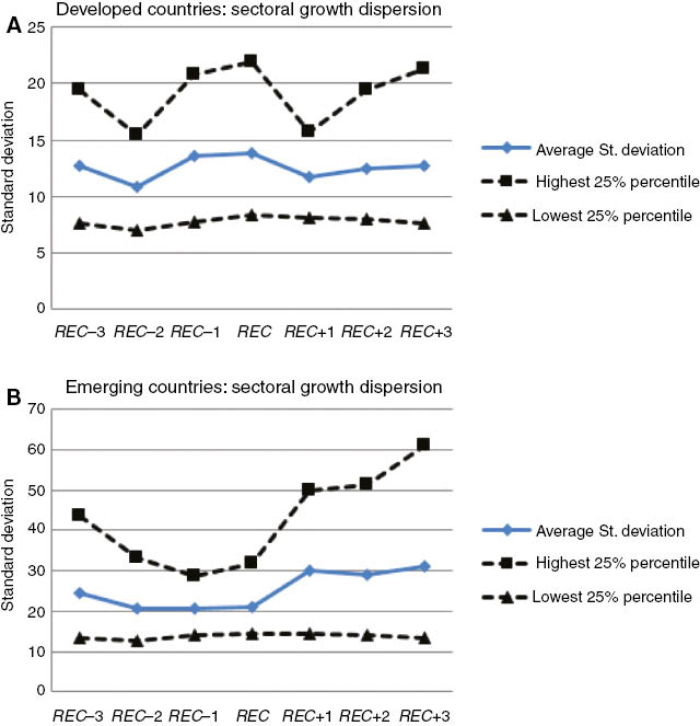
Standard deviation of VA growth across industries.
These results point to a marked difference between the behavior of sectors across the two groups of countries: while EM markets display more dispersion in VA growth rates, this dispersion behaves counter-cyclically for DV countries and pro-cyclically for EM markets.
3.3 Peaks, troughs, and concordance
We now characterize recessions using a turning points methodology that allows us to unveil the degree of comovement of industries not only for recession episodes, but for all the different stages of the business cycle. We identify turning points in industry cycles following Harding (2002), which is an annual variant of the quarterly Harding and Pagan (2002) algorithm. We apply the algorithm on the log levels of industrial VA. For a given series yt, a peak (trough) is identified at time t if yt is higher (lower) than the observations in the preceding and the following year. In particular, a peak is identified in a time series
Following Harding and Pagan (2002), we then obtain a measure of comovement, known as the concordance index. This index measures the fraction of time two series are in the same phase of the cycle. We make use of this index in three different ways. First, we measure the concordance of phases between an industry and the aggregate business cycle of a given country. This is measured by:
Where Si,x,t and Sx,t are binary variables capturing expansion and contraction phases of industry i of country x and the aggregate of country x, respectively. Secondly, we measure the concordance of phases between two industries of the same country by:
where i, j are combinations of industries where i≠j and n is the total number of pairwise combinations of industries i and j. Therefore, Si,x,t and Sj,x,t are binary variables capturing expansion and contraction phases of industries i and j of country x, respectively.
Finally, we measure the concordance of phases between the same industry, i, across two DV countries or two EM, respectively. The index is estimated across all possible country pairs, n:
where x, y are combinations of industries where x≠y. Therefore, Si,x,t and Si,y,t are binary variables capturing expansion and contraction phases of industry i of country x and y, respectively.
Table 3 summarizes the key characteristics of business cycles for DV and EM countries in terms of duration and amplitude using aggregate GDP data. In terms of duration, differences between the two groups are small. EM countries tend to have slightly longer contractions and expansions, whereas cycles are mildly more asymmetric for DV countries (i.e. differences in the duration of contractions and expansions are larger). The main difference arise in the amplitude of the cycles. As commented above, both contractions and expansions tend to be much larger for EM countries, leading to much higher business cycle volatility.
Duration and amplitude of aggregate cycles.
| Duration | Amplitude | |||||||||
|---|---|---|---|---|---|---|---|---|---|---|
| Contraction | Expansion | Asymmetry | Contraction | Expansion | ||||||
| DV | EM | DV | EM | DV | EM | DV | EM | DV | EM | |
| Mean | 1.3 | 1.5 | 7.7 | 8.1 | 6.6 | 6.2 | –1.6 | –6.2 | 27.8 | 45.7 |
| Median | 1.0 | 1.5 | 7.1 | 8.0 | 6.4 | 5.3 | –1.5 | –4.4 | 27.3 | 42.3 |
| Min | 1.0 | 1.0 | 4.0 | 4.0 | 2.4 | 1.5 | –3.6 | –14.3 | 11.9 | 20.6 |
| Max | 2.0 | 2.8 | 10.0 | 14.5 | 10.0 | 10.0 | –0.2 | –0.8 | 58.9 | 75.0 |
| Std. dev. | 0.3 | 0.5 | 2.1 | 3.1 | 2.7 | 3.2 | 1.0 | 4.0 | 12.8 | 19.7 |
Table 4 presents the concordance index for industries within countries. The results capture the percentage of time an industry is in the same phase of the cycle as the aggregate or another industry. The first set of columns estimates the index between industries and the aggregate as in equation (1), and the second set estimates the pairwise index as in equation (2). Both sets of results are then aggregated for presentation. In DV countries, on average, a randomly selected industry will be in the same phase as the aggregate economy 61.4% of the time. This number is very similar for EM economies (63.2%). The same conclusion can be obtained when looking at the average pairwise concordance indexes. There are no substantial differences between the two groups of countries. Interestingly, the countries showing the highest degree of concordance are South Korea and the US.
Concordance indexes within countries.
| Country | Concordance indexes between aggregate and individual industry cycles | Concordance indexes between individual industry cycles | ||||||||
|---|---|---|---|---|---|---|---|---|---|---|
| Mean | Median | Min | Max | Std. dev. | Mean | Median | Min | Max | Std. dev. | |
| Australia | 0.682 | 0.688 | 0.406 | 0.955 | 0.103 | 0.610 | 0.625 | 0.281 | 0.938 | 0.117 |
| Austria | 0.638 | 0.680 | 0.419 | 0.788 | 0.105 | 0.586 | 0.593 | 0.280 | 0.840 | 0.108 |
| Belgium | 0.587 | 0.594 | 0.438 | 0.750 | 0.101 | 0.578 | 0.594 | 0.375 | 0.781 | 0.094 |
| Canada | 0.684 | 0.667 | 0.485 | 0.848 | 0.100 | 0.625 | 0.606 | 0.364 | 0.909 | 0.102 |
| Denmark | 0.675 | 0.682 | 0.455 | 0.955 | 0.116 | 0.586 | 0.591 | 0.227 | 0.909 | 0.131 |
| Finland | 0.615 | 0.606 | 0.485 | 0.818 | 0.110 | 0.573 | 0.576 | 0.303 | 0.848 | 0.103 |
| France | 0.555 | 0.576 | 0.212 | 0.758 | 0.146 | 0.582 | 0.576 | 0.303 | 0.879 | 0.102 |
| West Germany | 0.631 | 0.682 | 0.227 | 0.955 | 0.187 | 0.599 | 0.591 | 0.227 | 0.909 | 0.136 |
| Greece | 0.610 | 0.621 | 0.345 | 0.826 | 0.116 | 0.559 | 0.552 | 0.310 | 0.828 | 0.103 |
| Ireland | 0.609 | 0.594 | 0.400 | 0.813 | 0.117 | 0.557 | 0.563 | 0.200 | 0.920 | 0.126 |
| Israel | 0.601 | 0.606 | 0.455 | 0.758 | 0.082 | 0.651 | 0.655 | 0.444 | 0.909 | 0.088 |
| Italy | 0.538 | 0.530 | 0.424 | 0.727 | 0.093 | 0.556 | 0.545 | 0.273 | 0.879 | 0.103 |
| Japan | 0.615 | 0.606 | 0.303 | 0.848 | 0.139 | 0.644 | 0.636 | 0.303 | 0.939 | 0.116 |
| Netherlands | 0.585 | 0.625 | 0.250 | 0.875 | 0.139 | 0.566 | 0.542 | 0.250 | 0.958 | 0.123 |
| New Zealand | 0.562 | 0.611 | 0.333 | 0.765 | 0.109 | 0.574 | 0.556 | 0.222 | 0.889 | 0.135 |
| Norway | 0.504 | 0.516 | 0.188 | 0.656 | 0.112 | 0.514 | 0.522 | 0.217 | 0.826 | 0.110 |
| Portugal | 0.598 | 0.576 | 0.333 | 0.788 | 0.098 | 0.549 | 0.545 | 0.273 | 0.788 | 0.093 |
| Singapore | 0.631 | 0.636 | 0.394 | 0.909 | 0.154 | 0.579 | 0.576 | 0.303 | 0.879 | 0.098 |
| Spain | 0.612 | 0.636 | 0.424 | 0.848 | 0.100 | 0.588 | 0.576 | 0.273 | 0.879 | 0.101 |
| Sweden | 0.611 | 0.613 | 0.290 | 0.774 | 0.129 | 0.581 | 0.581 | 0.258 | 0.871 | 0.109 |
| UK | 0.617 | 0.606 | 0.346 | 0.848 | 0.106 | 0.612 | 0.615 | 0.269 | 0.879 | 0.107 |
| US | 0.745 | 0.758 | 0.333 | 0.909 | 0.136 | 0.671 | 0.697 | 0.212 | 0.939 | 0.138 |
| Total DV | 0.614 | 0.611 | 0.505 | 0.745 | 0.052 | 0.588 | 0.582 | 0.514 | 0.671 | 0.036 |
| Chile | 0.595 | 0.586 | 0.379 | 0.828 | 0.108 | 0.582 | 0.586 | 0.310 | 0.793 | 0.090 |
| Colombia | 0.587 | 0.600 | 0.233 | 0.867 | 0.116 | |||||
| Ecuador | 0.645 | 0.652 | 0.455 | 0.818 | 0.088 | 0.592 | 0.576 | 0.333 | 0.879 | 0.091 |
| Honk Kong | 0.573 | 0.533 | 0.464 | 0.833 | 0.116 | 0.568 | 0.567 | 0.333 | 0.867 | 0.121 |
| Hungary | 0.633 | 0.636 | 0.455 | 0.848 | 0.109 | 0.621 | 0.613 | 0.387 | 0.909 | 0.105 |
| India | 0.548 | 0.545 | 0.364 | 0.697 | 0.080 | 0.575 | 0.576 | 0.333 | 0.848 | 0.086 |
| Indonesia | 0.653 | 0.667 | 0.515 | 0.759 | 0.070 | 0.567 | 0.576 | 0.364 | 0.848 | 0.096 |
| Iran | 0.655 | 0.652 | 0.333 | 0.818 | 0.100 | 0.647 | 0.636 | 0.364 | 0.909 | 0.106 |
| Jordan | 0.529 | 0.542 | 0.375 | 0.792 | 0.097 | 0.537 | 0.542 | 0.292 | 0.875 | 0.119 |
| Korea | 0.750 | 0.781 | 0.531 | 0.938 | 0.109 | 0.680 | 0.688 | 0.406 | 0.906 | 0.094 |
| Malaysia | 0.704 | 0.727 | 0.515 | 0.909 | 0.110 | 0.601 | 0.606 | 0.364 | 0.848 | 0.095 |
| Malta | 0.657 | 0.654 | 0.455 | 0.864 | 0.109 | 0.555 | 0.545 | 0.273 | 0.818 | 0.107 |
| Panama | 0.572 | 0.586 | 0.355 | 0.773 | 0.092 | 0.571 | 0.581 | 0.273 | 0.818 | 0.098 |
| Turkey | 0.656 | 0.643 | 0.464 | 0.786 | 0.096 | 0.563 | 0.571 | 0.286 | 0.786 | 0.099 |
| Zimbabwe | 0.678 | 0.692 | 0.538 | 0.808 | 0.081 | 0.666 | 0.654 | 0.423 | 0.885 | 0.092 |
| Total EM | 0.632 | 0.649 | 0.529 | 0.750 | 0.062 | 0.594 | 0.582 | 0.537 | 0.680 | 0.042 |
| p-Value (variance) | 0.4850 | 0.5415 | ||||||||
| p-Value (mean) | 0.3518 | 0.6474 | ||||||||
Colombia only faced one expansion at the aggregate level.
Table 5 presents the results of concordance index as in equation (3) looking at comovement across the same industry between countries. These are concordance indexes for all the pairwise combinations of the same industry across DV and EM countries. They capture the percentage of time two same industries in two different DV or EM countries are in the same cyclical phase. The results are then grouped by industry. They suggest that same industries across DV countries are more often in the same phase than industries across EM countries. This is especially the case for industries that are heavily used for intermediate inputs such as chemical products. While differences are of a small order of magnitude, they are highly statistically significant, and they point out that stronger inter-industry trade linkages may be driving these results.[11]
Concordance indexes between industries across countries.
| ISIC | Developed countries | Emerging countries | ||||||||
|---|---|---|---|---|---|---|---|---|---|---|
| Mean | Median | Min | Max | Std. dev. | Mean | Median | Min | Max | Std. dev. | |
| 311 | 0.605 | 0.611 | 0.278 | 0.903 | 0.105 | 0.541 | 0.548 | 0.250 | 0.769 | 0.098 |
| 313 | 0.552 | 0.556 | 0.167 | 0.862 | 0.106 | 0.540 | 0.560 | 0.333 | 0.700 | 0.086 |
| 314 | 0.523 | 0.542 | 0.227 | 0.758 | 0.103 | 0.532 | 0.537 | 0.321 | 0.731 | 0.101 |
| 321 | 0.574 | 0.586 | 0.222 | 0.818 | 0.116 | 0.543 | 0.538 | 0.300 | 0.808 | 0.090 |
| 322 | 0.545 | 0.548 | 0.292 | 0.871 | 0.098 | 0.526 | 0.538 | 0.267 | 0.750 | 0.095 |
| 323 | 0.549 | 0.552 | 0.222 | 0.788 | 0.097 | 0.510 | 0.500 | 0.273 | 0.818 | 0.106 |
| 324 | 0.516 | 0.516 | 0.227 | 0.818 | 0.094 | 0.507 | 0.522 | 0.250 | 0.692 | 0.099 |
| 331 | 0.573 | 0.576 | 0.333 | 0.939 | 0.100 | 0.515 | 0.515 | 0.208 | 0.731 | 0.108 |
| 332 | 0.544 | 0.545 | 0.333 | 0.778 | 0.096 | 0.516 | 0.531 | 0.261 | 0.773 | 0.098 |
| 341 | 0.606 | 0.594 | 0.222 | 0.909 | 0.112 | 0.554 | 0.552 | 0.355 | 0.793 | 0.101 |
| 342 | 0.610 | 0.611 | 0.273 | 0.875 | 0.117 | 0.572 | 0.577 | 0.321 | 0.828 | 0.098 |
| 351 | 0.650 | 0.654 | 0.391 | 0.909 | 0.095 | 0.535 | 0.538 | 0.292 | 0.844 | 0.106 |
| 352 | 0.651 | 0.667 | 0.344 | 0.909 | 0.114 | 0.581 | 0.571 | 0.333 | 0.864 | 0.116 |
| 353 | 0.533 | 0.533 | 0.273 | 0.867 | 0.099 | 0.534 | 0.563 | 0.250 | 0.750 | 0.115 |
| 354 | 0.543 | 0.545 | 0.222 | 0.889 | 0.117 | 0.471 | 0.466 | 0.429 | 0.536 | 0.042 |
| 355 | 0.577 | 0.576 | 0.313 | 0.889 | 0.106 | 0.526 | 0.524 | 0.276 | 0.750 | 0.109 |
| 356 | 0.609 | 0.613 | 0.278 | 0.909 | 0.121 | 0.557 | 0.567 | 0.321 | 0.742 | 0.095 |
| 361 | 0.572 | 0.563 | 0.310 | 0.864 | 0.097 | 0.531 | 0.538 | 0.300 | 0.821 | 0.100 |
| 362 | 0.592 | 0.594 | 0.278 | 0.864 | 0.104 | 0.543 | 0.547 | 0.292 | 0.800 | 0.097 |
| 369 | 0.595 | 0.591 | 0.333 | 0.909 | 0.100 | 0.536 | 0.538 | 0.235 | 0.758 | 0.097 |
| 371 | 0.571 | 0.576 | 0.222 | 0.818 | 0.112 | 0.537 | 0.540 | 0.333 | 0.786 | 0.093 |
| 372 | 0.569 | 0.581 | 0.227 | 0.813 | 0.098 | 0.512 | 0.508 | 0.300 | 0.731 | 0.092 |
| 381 | 0.587 | 0.591 | 0.227 | 0.864 | 0.116 | 0.543 | 0.538 | 0.217 | 0.781 | 0.106 |
| 382 | 0.551 | 0.545 | 0.318 | 0.848 | 0.095 | 0.533 | 0.538 | 0.231 | 0.750 | 0.101 |
| 383 | 0.599 | 0.594 | 0.355 | 0.935 | 0.097 | 0.596 | 0.600 | 0.400 | 0.813 | 0.079 |
| 384 | 0.536 | 0.545 | 0.278 | 0.778 | 0.105 | 0.553 | 0.545 | 0.333 | 0.727 | 0.093 |
| 385 | 0.553 | 0.545 | 0.273 | 0.818 | 0.105 | 0.528 | 0.538 | 0.333 | 0.760 | 0.090 |
| 390 | 0.529 | 0.545 | 0.227 | 0.758 | 0.094 | 0.528 | 0.536 | 0.300 | 0.762 | 0.099 |
| Average | 0.574 | 0.576 | 0.167 | 0.939 | 0.110 | 0.539 | 0.542 | 0.208 | 0.864 | 0.100 |
| p-Value (variance) | 0.0519 | |||||||||
| p-Value (mean) | 0.0000 | |||||||||
4 Industry behavior around recessions: methods and results
For 7-years intervals centered at the first year of recession, our analysis focuses on three approaches. First, we look at economic activity of various sectors and their shares in total industry. Second, we analyze sectoral concentration, and third, we implement a shift-share analysis, as well as the Olley-Pakes(OP) decomposition.
4.1 Sectoral activity and shares
Our descriptive analysis will now focus on how economic activity at a sectoral level behaves around recession episodes. We are particularly interested on the evolution of VA, employment, productivity, and VA and employment shares as indicators of sectoral reallocation. Given the definition of a recession discussed above, we plot the evolution of these variables for the 7 years that span the 3 pre-recession and the 3 post-recession years (REC–3 to REC+3). The plots contain the average behavior of the variable across all recessions for each country. We analyzed the results for each country and industry. However, to facilitate presentation, we only report averages for the two groups of DV and EM countries.
Furthermore, because presentation and interpretation is obscured by the large number of industries and variables available, we also collapse industries in four groups depending on their (labor) productivity level. This is because a question of interest, rather than the specific branches themselves, is whether activity reallocates between branches with different productivity characteristics. We classify industries into the following four categories: High, Medium-High, Medium-Low, and Low productivity. We used two different methodologies for this classification. The first simply ranks industries for each country (within) in terms of their productivity levels and assigns them into their corresponding groups by quartiles. The second methodology, rather than using a within country criterion, ranks industries by their level of productivity relative to the same industry in the US. That is, this classification normalizes by the standard dispersion in productivity that exists across different industries because of technical characteristics using the US as the reference country. Although there are some non-negligible differences between these two classification methods regarding the composition of branches, both gave similar results in terms of their behavior around recession points. For this reason, we report here only the results using the first method. Also, this classification is perhaps more interesting as it ranks industries according to their within country productivity level and is hence compatible with a definition of comparative advantage.[12] All variables were then averaged out for the industries in each group for both groups of DV and EM countries.
Moreover, Rajan and Zingales (1998) identify the level of an industry’s dependence on external finance (the difference between investments and cash generated by operations) from data on US firms.[13] We make use of this index and collapse industries in four groups depending on the level of EFD: Low to No EFD, Medium-Low, Medium-High, and High EFD. Given that their index provides a measure of an industry’s EFD in the 1980s, we assume that the same ordering will hold for the specific time period under examination in this study, 1970–2002. Importantly, we want to observe whether the depth of the recession and the speed of recovery change for different levels of financial dependency, and whether this result is different between DV and developing countries. All variables were then averaged out for the industries in each group for both groups of DV and EM countries.
Finally, we distinguish between normal and financial recessions by externally identifying banking crises using Reinhart and Rogoff (2008), and compare those episodes between DV and EM economies. From the 120 recessions analyzed in this study, 29 were identified as financial recessions, among which 19 took place in the DV economies and the remaining 10 occurred in EM markets. Appendix B shows the countries and years for which financial recessions took place.
We now present the results grouping industries firstly by levels of productivity and, secondly, by levels of EFD. We then distinguish, on the one hand, between DV and EM economies, and on the other hand, between normal and financial recessions.[14]
4.1.1 Developed versus emerging economies
4.1.1.1 By levels of productivity for each group of countries
Figure 2 shows the evolution of averaged VA growth from REC–3 to REC+3 for DV and EM countries. Both groups of countries display a V shaped pattern at the REC point. The amplitude of the cycle is larger for EM markets for all groups of productivity levels. Note that, at t=REC, the lower the productivity level of an industry in DV countries the higher the contraction it will face. When comparing REC–3 to REC+3 values, we can see that neither EM nor DV economies recover to pre-recession rates within the 3 years following the recession. Despite that fact, some notable differences exist. EM markets generally face larger contractions than the DV countries, except for the medium-high productivity level group. Moreover, when comparing pre- to post-recession growth rates, while the two highly productive groups of industries face the largest drops in VA growth in DV countries, in the EM economies it is the two lowest productive groups that seem to be affected the most by recession episodes in terms of recovery. The differences observed between DV and EM are strongly significant at the 1% significance level, except for the high productivity group which suggests that the average VA growth in EM countries will be higher than the one in DV with a significance level of 10%.
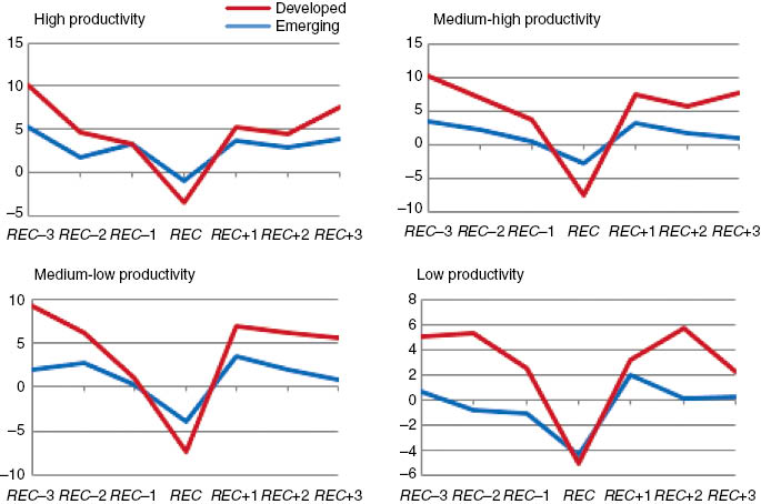
Average VA growth per level of productivity for developed and emerging countries.
Similarly, Figure 3 displays the evolution of averaged employment growth from REC–3 to REC+3 for DV and EM countries and results point to strongly significant differences between DV and EM markets at the 5% significance level for all groups of productivity levels. Both groups of countries display a V shaped pattern around the recession time period, although the amplitude of the cycle is larger for DV countries. Moreover, the recovery in employment is much stronger for EM than for DV economies, suggesting a higher degree of real wage flexibility in EM economies.[15] For the majority of the groups, the deepest contraction is observed the year of the recession. However, notable exceptions exist. On the one hand, the high productivity group of the EM markets does not face negative growth throughout the 7 years of analysis and on the other hand, the low productivity group of the DV countries displays negative growth from REC–3 to REC+3. Importantly, when comparing pre- to post-recession values, this figure shows that on average, the majority of manufacturing sectors in DV countries face very persistent employment losses after a recession. The opposite is true for the EM markets, as for any given productivity level, industries do on average recover to higher growth rates after the recession episode. Interestingly, while the two lowest productivity groups of the EM markets face the largest contractions in VA growth, they face the largest expansions in employment growth, although the latter are bigger than the former. This means that post-recession productivity growth has fallen, which is in line with the results from Figure 4.
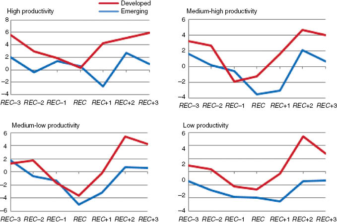
Average employment growth per level of productivity for developed and emerging countries.
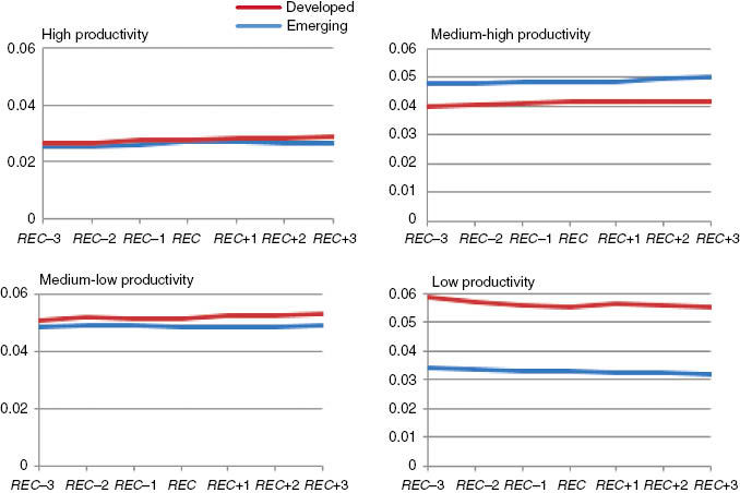
Average productivity growth per level of productivity for developed and emerging countries.
Overall, in DV countries by REC+3 productivity growth has returned to its pre-recession rates. In contrast, for EM markets by REC+3 productivity growth remains below its pre-recession growth rates for all productivity groups except for medium-high, which is also the only group for which results are found to be statistically significant at the 10% significance level.
We also look at the relative dispersion between the high and low productivity groups and the two middle productive groups for VA, Employment and Productivity growth.[16] Several results stand out. The relative dispersion is higher between high and low productivity groups especially for DV countries. For the EM countries, the relative dispersion is high at REC–3 and REC+3 and falls substantially during the 2 years window around the recession period. For the medium groups, fluctuations are overall around zero. For employment growth, the relative dispersion of the high and low productive groups increases during REC periods for DV countries and falls substantially during the recovery years. For EM this difference shows a constant trend from REC–3 to REC+1, when it then faces a substantial drop in REC+2 before increasing back to its previous levels. Similarly to VA growth dispersion, the medium groups for both DV and EM markets fluctuate around zero. Finally, for the relative dispersion in productivity growth for the high and low productive groups the dispersion decreases before and during recession episodes for DV countries and increases substantially the three following years. The dispersion in EM countries reaches similar levels to the ones observed for DV 3 years after the recession. Importantly however, the relative dispersion cannot highlight different types of dynamics. For instance, the difference can be negative because one group shrinks and the other grows, or because one shrinks more than the other. Qualitatively, both cases are different, although they may display the same type of dispersion.
Figure 5 shows the evolution of averaged VA shares per level of productivity. Shares in general do not display any marked variation around the recession date. Some underlying trends appear to be dominating, especially for the DV countries. But, overall, in DV countries there seems to be a very slight redistribution of VA shares from the lowest productivity group to the three remaining groups, albeit very small. The EM economies are not characterized by any restructuring in VA shares after a recession episode. A very similar picture arises from the evolution of employment shares (Figure 6). While for the average VA share the differences are strongly significant between DV and EM countries for all groups of productivity, this is not the case for the high and medium-low productivity groups when comparing the average employment shares from REC–3 to REC+3.

Average VA share per level of productivity for developed and emerging countries.
Average employment share per level of productivity for developed and emerging countries.
Finally, there is clear relationship between industrial productivity level and the distribution of VA and employment shares for EM countries. In particular, the higher the productivity level of an industry the higher the average level of VA shares and the lower the average level of employment shares. As shown later, this could be a consequence of higher sectoral concentration, or specialization, in EM than in DV markets.
4.1.1.2 By level of EFD
The amplitude of the cycle is larger for EM markets, independently of the level of EFD of the industries (Figure 7). When comparing pre- to post-recession values, overall, EM countries face large and persistent output losses, except for the group of industries that have medium-high EFD. For the DV countries, the only group facing gains in VA growth rates is the Low to No EFD, for which recovery occurs within the 3 years following the recession. The two groups with the highest EFD also face the largest contractions from REC–3 to REC+3 (≈2.4%). Moreover, industries with high dependence on external finance face a larger contraction in VA growth in both DV and EM countries. This result is in line with the ones found in Braun and Larrain (2005). All differences observed in the average evolution of VA growth between DV and EM countries are strongly significant for all groups of EFD.[17]
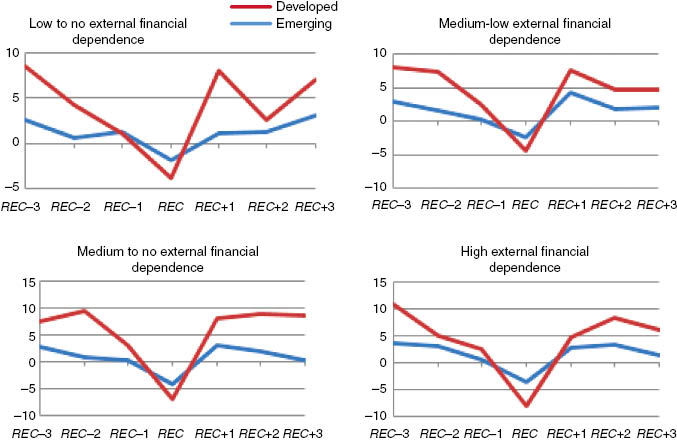
Average VA growth per level of external financial dependence (EFD) for developed and emerging countries.
4.1.2 Normal versus financial recessions
In this part we compare normal and financial recessions. Note that to compare results between the previous and the current analysis, one will have to look at the average evolution for all countries and all recessions. However, results are likely to present slight differences as averages are taken by country and not by the number of recessions or industries within a country. In other words, because we assume that countries in our sample are equally important we do not estimate weighted averages to account for the number of recessions in each industry and each category (productivity level or EFD). For instance, because of missing data one country might have only four industries in each grouping instead of seven, which would be the case for a country that has no missing industries. If we were to perform a weighted average to account for the number of industries in each grouping, we would be assuming that industries in the former country are more “important” than industries in the latter. The same would hold for the number of recessions.
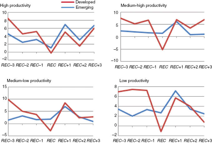
Figure 8 shows the evolution of average VA growth per level of productivity from REC–3 to REC+3 for all countries, when normal or financial recessions occur. For any given group of productivity level, we can see that contractions are larger for the case of financial recessions. Moreover, those types of episodes display a W shaped pattern, as growth at REC+1 is at higher levels than pre-recession, but during the following 2 years growth falls to lower levels. Therefore, when comparing REC–3 to REC+3 values, all industries seem to face losses in VA levels, except from those that have low productivity levels. This is the only group that recovers from financial recessions within 3 years. For normal recessions, the recovery is even slower as none of the four groups displays higher post-recession than pre-recession growth. Therefore, whatever the productivity level when normal recessions occur, industries face losses in VA. This result is also supported by Reinhart and Rogoff (2009b) who found that during crises, EM markets face a sharper fall in real GDP growth but a somewhat faster comeback to growth than advanced economies. Similar results are also presented by Calderón and Fuentes (2010). The observed differences are only weakly statistically significant. For the low productivity group, the significance tests suggests that the average VA growth is higher during normal than financial recessions with a p-value=0.0706.
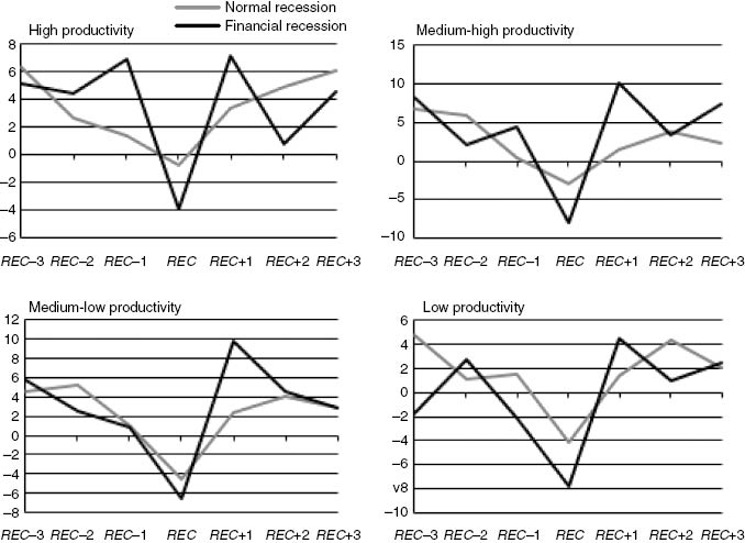
Average VA growth per level of productivity, normal versus financial recessions.
Figure 9 presents the results for industries ranked by level of financial dependence. Although results are not statistically significant, some interesting patterns arise. As seen before, the amplitude of the cycle is larger for financial recessions. Overall, industries with high EFD face larger contractions in VA growth the year of the financial crises, with contractions being larger for the case of financial recessions. Interestingly, and somehow puzzling, in industries with high EFD the recovery is faster in the case of financial recessions. This result is perhaps consistent with the evidence presented in the work by Calvo, Izquierdo, and Talvi (2006) on “phoenix miracles,” defined as rapid output recovery from financial crises, accompanied by the absence of credit recovery.
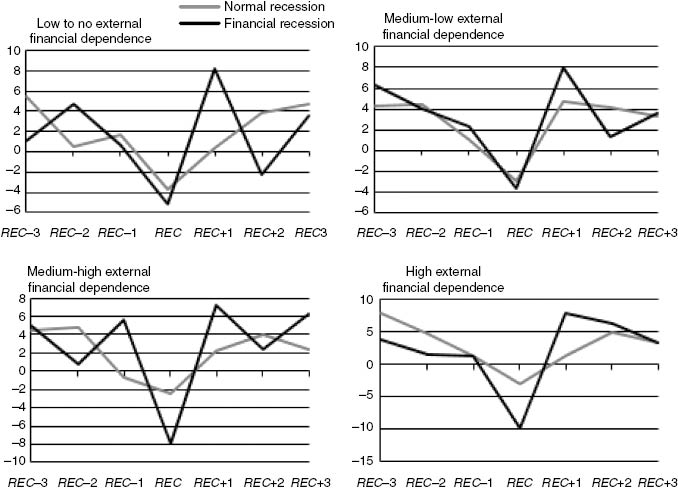
Average VA growth per level of external financial dependence (EFD), normal versus financial recessions.
4.2 Sectoral concentration/specialization: Gini and HHI indexes
We also examined whether recessions are associated with any significant changes in the degree of concentration of VA and employment. We can interpret this concentration as “specialization” as in Imbs and Wacziarg (2003), that is, whether a significant proportion of output (inputs) in the economy is being produced (used) by a few industries. By looking at VA and employment concentration, we can also infer the dispersion of productivity across industries. Whether recessions are associated with greater or lower specialization, of course, will depend on institutions, availability of credit, labor market frictions, changes in the composition of demand, openness, etc. We make use of two different measures: the Gini coefficient and the Herfindahl-Hirschman index (HHI).
The Gini coefficient uses information on how VA and Employment shares are distributed across the different industries. Employment shares have commonly been used in the empirical literature concerning sectoral specialization as a measure of sector size. However, making use of sectoral VA shares helps generalizing the evidence based on sectoral labor inputs.
A simple expression for the Gini index is based on the covariance between the ranked shares of VA or employment by industry, SR, and the rank that the industry occupies in the distribution of VA or Employment share, F. This rank takes a value between zero for the lowest VA or Employment share and one for the highest. The Gini index, varying between 0 for lowest and 1 for highest inequality, is then defined as:
where S̅R is the average VA or Employment share.
The HHI is another indicator of the level of concentration/specialization among industries in a sector used in the industrial organization literature. It is defined as the sum of the squared market shares of each industry branch in the sector. Again, we made use of both VA shares and employment shares to obtain the HHI. A decrease in the HHI indicates a decrease in concentration (more diversification). The expression for HHI is then:
where Si is the share (of VA or employment) of branch i in the manufacturing sector, and N is the number of branches. The HHI (H) ranges from 1/N to one. If all branches have an equal share, the reciprocal of the index shows the number of industries in the sector. The HHI takes into account the relative size and distribution of the industries in a sector and approaches zero when a sector consists of a large number of industries of relatively equal size. The HHI increases both as the number of industries in the market decreases and as the disparity in size between those industries increases. Because of this dependence on N, and given that countries in our sample have unequal numbers of branches, we prefer to use the normalized HHI:
While the H ranges from 1/N to 1, H* ranges from 0 to 1 regardless of the number of branches considered.
Tables 6 and 7 present the Gini and HHI coefficients for sectoral VA and employment shares for DV and EM economies, respectively. Overall, it is obvious that changes in sectoral specialization/concentration are modest, as magnitude changes are in general relatively small. While the differences obtained in the Gini coefficient are statistically insignificant, the ones in the HHI between DV and EM are strongly statistically significant for both VA and employment shares.[18]
Average Gini and HHI coefficients for developed countries.
| Index | Variable | REC-3 | REC-2 | REC-1 | REC | REC+1 | REC+2 | REC+3 |
|---|---|---|---|---|---|---|---|---|
| Gini | Employment | 0.50395 | 0.50625 | 0.50712 | 0.50640 | 0.50729 | 0.50955 | 0.51191 |
| VA | 0.48026 | 0.48185 | 0.48565 | 0.48816 | 0.49204 | 0.49320 | 0.49269 | |
| HHI | Employment | 0.04022 | 0.04078 | 0.04107 | 0.04022 | 0.04027 | 0.04166 | 0.04264 |
| VA | 0.03673 | 0.03746 | 0.03847 | 0.03829 | 0.03941 | 0.03957 | 0.03922 |
Average Gini and HHI coefficients for emerging countries.
| Index | Variable | REC–3 | REC–2 | REC–1 | REC | REC+1 | REC+2 | REC+3 |
|---|---|---|---|---|---|---|---|---|
| Gini | Employment | 0.51989 | 0.51614 | 0.51493 | 0.51673 | 0.51699 | 0.51786 | 0.51629 |
| VA | 0.48860 | 0.48393 | 0.49229 | 0.50170 | 0.50452 | 0.50702 | 0.50300 | |
| HHI | Employment | 0.05830 | 0.05719 | 0.05635 | 0.05808 | 0.05965 | 0.05954 | 0.05850 |
| VA | 0.04720 | 0.04517 | 0.04635 | 0.05133 | 0.05543 | 0.05467 | 0.05179 |
Some important patterns can be observed. When looking at the Gini coefficient, two main conclusions can be drawn. Firstly, the manufacturing sector of DV countries is less specialized around recessions for both VA and employment, when compared to EM markets. Secondly, for both DV and EM countries, employment shares are in general more unequally distributed than VA shares. Although for EM markets the gap between those two measures is marginally larger the 3 years before the recession, at t=REC and the 3 years following the recession this gap becomes larger for the DV economies. This implies that before the recession, productivity is more concentrated in EM than in DV countries. However, at the recession year and the 3 years that follow, productivity becomes more concentrated in DV than in EM countries. Moreover, when looking at the HHI index, results indicate that, with the exception of a few countries like Singapore, Ecuador and Panama,[19] all countries display low concentration (HHI<0.1) whether using sectoral employment or VA shares. Furthermore, when using either the sectoral VA or employment shares to estimate the HHI, concentration is significantly higher among EM markets than it is among DV countries. Finally, as for the Gini coefficient, employment shares are in general more unequally distributed than VA shares. Therefore, productivity is more concentrated in EM than in DV countries, as the gap between the two measures (VA and employment shares) is larger for the former group of countries throughout the 7 years of analysis. Although the gap is slightly higher for EM markets, after a recession this closes down much more for EM than for DV countries.
4.3 Accounting for structural change: a shift-share analysis and sector misallocation
Shift-share analysis is a descriptive technique to analyze the sources of productivity growth. First proposed by Maddison (1952), it shows how aggregate growth is mechanically linked to differential growth of labor productivity and the reallocation of labor between industries. It has been widely applied for analyzing the effect of industrial structural change on productivity growth (e.g. Fagerberg 2000; Peneder 2003) and microeconomic evidence on the sources of growth (e.g. Foster, Haltiwanger, and Krizan 2001).
Let us define LP=Labor Productivity, VA=Value Added, L=Labor input, and i=industry index with i=(1, …, N). Then,
Define
Defining ΔLP=LP1–LP0, ΔS=S1–S0 and using equation (8), we have:
We can express (9) in growth rate form:
The percentage change in labor productivity between time t=0 and t=1 is hence decomposed into three distinct effects. The first component of eq. (10) is the so-called “static-shift effect” and it measures the impact that changes in the allocation of labor between industries have on productivity growth. It will be positive if the share of high productivity industries increases in total employment by attracting more labor resources at the expense of low productivity industries. The second term in (10) is the so-called “within-shift effect” and it measures the change in productivity that would have prevailed if no change in sectoral shares had taken place between 0 and 1. That is, it measures productivity gains that have occurred only within industries. Finally, the third effect is the so-called “dynamic-shift effect.” It captures interactions between changes in sectoral structure and within productivity effects. This effect will be positive if changes in shares favor those industries where productivity is growing. Thus, the “dynamic-shift effect” reflects whether a country reallocates its labor resources towards industries with fast growing productivity.[20]
Table 8 summarizes the results obtained from the shift-share analysis. It reports the three effects, namely the within, the static, and the dynamic-shift effects, for normal times, recessions and financial recessions, distinguishing DM and EM.[21]
Shift-share analysis.
| Within-shift effect (in%) | Dynamic-shift effect (in%) | Static-shift effect (in%) | ||||
|---|---|---|---|---|---|---|
| Mean | Std. dev. | Mean | Std. dev. | Mean | Std. dev. | |
| All countries | ||||||
| Normal times | 85.50 | 157.30 | 22.99055 | 134.5619 | –8.58101 | 179.8772 |
| REC periods | 122.8573 | 152.9548 | –20.9907 | 93.05781 | –2.47268 | 119.7475 |
| Financial crises | 108.5471 | 49.18969 | –6.46949 | 38.55118 | –2.07761 | 63.79008 |
| DV | ||||||
| Normal times | 87.92 | 120.3435 | –11.81 | 51.29358 | 23.74 | 127.4078 |
| REC periods | 117.23 | 126.8893 | –12.33 | 64.17426 | –5.90 | 140.5117 |
| Financial crises | 98.40 | 13.32579 | –18.45 | 44.57083 | 20.06 | 37.70998 |
| EM | ||||||
| Normal times | 81.94493 | 204.6501 | 74.03437 | 194.7284 | –55.9793 | 234.101 |
| REC periods | 131.5201 | 191.7288 | –34.314 | 127.4939 | 2.793904 | 83.2368 |
| Financial crises | 122.5048 | 74.72375 | 10.00535 | 21.16383 | –32.5101 | 81.26425 |
Overall, the within-shift effect is positive for both DV and EM countries. This result implies that, on aggregate, reallocations of labor between industries (with different productivity levels) do not play an important effect on overall productivity growth. This effect appears to be dominating the structural components, which is in line with results reported in the literature.[22] It should be emphasized that, at this level of aggregation, all structural shifts between firms within branches will be included in the within effect. To the extent that little resource shift happens between very different branches, we would then expect the static-shift effect to be of a smaller magnitude. The other two effects, the static- and dynamic-shift effects, are more volatile and can be either positive or negative. One pattern that seems to distinguish DV and EM countries is that the dynamic-shift effect plays a more important role in the latter than in the former during recessions. Interestingly, the sign is reversed for this component for EM during financial crises. Finally, the static effect is negative in DV while positive in EM during recession periods, although the opposite is true during financial crises.
In summary, there does not seem to be a clear pattern between the structural components and the recession episodes. Sector-level reallocation does not seem to be associated with the state of the business cycle but rather with longer run trends. Thus, at this level of disaggregation at least, this contradicts theories predicting that, during recessions, there will be more restructuring (i.e. Hall 1991; Caballero and Hammour 1994). Nevertheless, restructuring at the firm level may still be substantial and reflected on within industry effects.
Another relevant issue is whether, for a given level of reallocation, resources are reallocated towards more productive industries. In order to assess this reallocation effect we implement the OP decomposition. There is another way of decomposing productivity which looks at misallocation. Define the aggregate productivity of an economy as P, which is simply the weighted sum of productivities of industries Pi, weighted by their employment shares Si. P can thus be decomposed in the following way:
where mean(Pi) is the un-weighted mean productivity and the second term is the OP term: the covariance between productivity and sector share. If this covariance is zero, then aggregate productivity is just the mean productivity of its industries. But if large industries have higher productivity, then labor is allocated to the more productive industries and the covariance is positive. Therefore, this is a measure of misallocation: if the OP term is high then resources are more efficiently allocated, if the OP term is negative or zero, then they are not efficiently allocated. Suppose cov(Pi, Si)=0.2, then this implies that aggregate productivity is 20% higher than if labor was randomly allocated between industries.
Figure 10 reports results for the OP decomposition. For DV countries the level of misallocation does not vary across different types of recessions. A slight upward trend can be observed from REC–3 to REC–3 both during financial crises and “normal” recessions. This trend is sustained for recession periods reducing the misallocation until 1 year after the recession occurs. In the following periods the covariance term remains practically constant. The same is observed for the case of financial crises but at a lower rate. Turning to EM economies, financial crises seem to lead to stronger misallocation 1–3 years after its occurrence. For normal recessions the pattern is very similar to the one observed for DV countries, although the trend is slightly more pronounced.
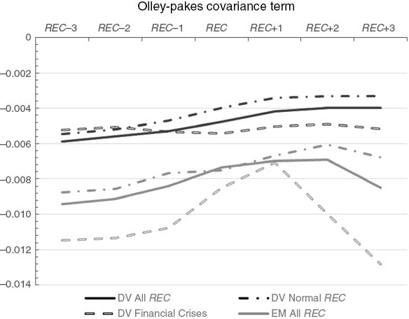
Olley-Pakes decomposition between DV and EM countries for normal times, recessions and financial crisis.
In summary, it appears that recessions do not lead to an improved allocation of resources between industries in the manufacturing sector. In EM, in fact, inter-industry misallocation significantly increases during episodes of financial crises.
5 Conclusions
We characterize the behavior of economies around recession periods at a disaggregate level by looking at data for 28 industrial branches for a set of 37 developed (DV) and Emerging (EM) countries. Industries are categorized in terms of their productivity level as well as their level of EFD. Based on those classifications, we look at the evolution of VA, employment, productivity, industrial concentration, and sectoral shares and distinguish between normal and financial recessions. Moreover, we look at the incidence of economy-wide versus industry-specific recessions as well as measures of the degree of industrial business cycle coordination. Finally, we decompose different sources of productivity growth and analyze their behavior during recessions. Although it is not possible to extract meaningful causal or structural interpretations from our results, they provide a set of stylized facts that are useful for both policy and model building.
Our results show that recessions tend to have only slightly higher incidence and duration in EM markets when compared with DV ones. However, the amplitude of these events in EM is much larger leading, in general, to much deeper output losses. There seems to be some evidence, albeit limited, that recessions tend to be more coordinated across manufacturing industries in DV countries than they are across the developing countries. The degree of business cycle comovement between industries at all stages of the business cycle is similar in both sets of countries. EM markets display a pro-cyclical dispersion of VA growth rates whereas this dispersion behaves counter-cyclically for DV countries. In general, we also see that the amplitude of the cycle for VA and productivity growth is larger for EM markets. The opposite is generally true for employment growth. The lower variability in employment in EM economies suggests a higher degree of real wage flexibility.
In DV countries, the two highly productive groups of industries display the slowest recovery in VA growth after a recession, while in the EM economies it is the two lowest productivity groups that appear more sluggish. Overall, productivity growth in DV countries tends to return to its pre-recession rates 3 years after the recession, while for EM it remains below its pre-recession rates for all productivity groups except for the medium-high, which is also the only group for which results are found to be statistically different. Industries with high dependence on external finance generally face higher contractions in VA growth the year of the recession, and those contractions are larger on the one hand for the EM countries when compared to DV economies and, on the other hand, in the case of financial crises.
Our findings also show that there is very little redistribution of economic activity across industries around recession episodes. Concentration of both VA and employment is higher among EM markets and, especially, when looking at employment shares. Finally, productivity growth is mostly driven by within-industry productivity gains, confirming previous aggregate evidence. However, the relation between recessions and productivity decomposition is not clear-cut. Using the Olly-Pakes decomposition we find that misallocation does not change significantly during recession episodes in DV economies. EM economies display similar dynamics with the exception of financial recessions, which are associated to sharp increases in misallocation. One could conclude with caution that at, this level of disaggregation, sector-level reallocation does not seem to be strongly associated with the state of the business cycle and in particular with recessions.
Acknowledgments
We thank an anonymous referee and the editor for very helpful comments on an earlier version of the paper. This work was supported by the Economic and Social Research Council [grant number ES/H00288X/1].
Appendix
List of industries.
| ISIC | Industries |
|---|---|
| 311 | Food products |
| 313 | Beverages |
| 314 | Tobacco |
| 321 | Textiles |
| 322 | Wearing apparel, except footwear |
| 323 | Leather products |
| 324 | Footwear, except rubber or plastic |
| 331 | Wood products, except furniture |
| 332 | Furniture, except metal |
| 341 | Paper and products |
| 342 | Printing and publishing |
| 351 | Industrial chemicals |
| 352 | Other chemicals |
| 353 | Petroleum refineries |
| 354 | Misc. petroleum and coal products |
| 355 | Rubber products |
| 356 | Plastic products |
| 361 | Pottery, china, earthenware |
| 362 | Glass and products |
| 369 | Other non-metallic mineral products |
| 371 | Iron and steel |
| 372 | Non-ferrous metals |
| 381 | Fabricated metal products |
| 382 | Machinery, except electrical |
| 383 | Machinery, electric |
| 384 | Transport equipment |
| 385 | Professional and scientific equipment |
| 390 | Other manufactured products |
Externally identified financial recessions.
| Country | Year of financial recession |
|---|---|
| Australia | 1991 |
| Denmark | 1988 |
| Ecuador | 1999 |
| Finland | 1991–1993 |
| Greece | 1993 |
| Honk-Kong | 1998 |
| Hungary | 1991–1993 |
| Indonesia | 1998 |
| Israel | 1977 |
| Italy | 1993 |
| Jordan | 1989 |
| Malaysia | 1985 |
| Norway | 1988 |
| Panama | 1988 |
| Spain | 1981 |
| Sweden | 1991–1993 |
| Turkey | 1994 |
| UK | 1974–1975, 1991 |
| US | 1991 |
References
Aghion, Philippe, George-Marios Angeletos, Abhijit Banerjee, and Kalina Manova. 2005. “Volatility and Growth: Credit Constraints and Productivity-Enhancing Investment.” NBER Working Papers No. 11349. Cambridge, Massachusetts, National Bureau of Economic Research.10.1093/acprof:oso/9780199248612.001.0001Search in Google Scholar
Aguiar, Mark, and Gita Gopinath. 2007. “Emerging Market Business Cycles: The Cycle Is the Trend.” Journal of Political Economy 115: 69–102.10.3386/w10734Search in Google Scholar
Arbache, Jorge S., and John Page. 2010. “How Fragile Is Africa’s Recent Growth?” Journal of African Economies 19 (1): 1–24.10.1093/jae/ejp017Search in Google Scholar
Barlevy, Gadi. 2007. “On the Cyclicality of Research and Development.” American Economic Review 97: 1131–1164.10.1257/aer.97.4.1131Search in Google Scholar
Baumol, William J., Sue A. B. Blackman, and Edward Wolff. 1985. “Unbalanced Growth Revisited: Asymptotic Stagnancy and New Evidence.” American Economic Review 75: 806–817.Search in Google Scholar
Braun, Matias, and Borja Larrain. 2005. “Finance and the Business Cycle: International, Inter-Industry Evidence.” The Journal of Finance 60 (3): 1097–1127.10.1111/j.1540-6261.2005.00757.xSearch in Google Scholar
Caballero, Ricardo J., and Mohamad L. Hammour. 1994. “The Cleansing Effects of Recessions.” American Economic Review 84: 1350–1368.10.3386/w3922Search in Google Scholar
Calderón, Cesar, and Rodrigo Fuentes. 2010. “Characterizing the Business Cycles of Emerging Economies.” The World Bank, Policy Research Working Paper Series No. 5343.10.1596/1813-9450-5343Search in Google Scholar
Calvo, Guillermo A., and Fabrizio Coricelli, and Pablo Ottonello. 2012. “Labor Market, Financial Crises and Inflation: Jobless and Wageless Recoveries.” NBER Working Papers 18480.10.3386/w18480Search in Google Scholar
Calvo, Guillermo, Alejandro Izquierdo, and Ernesto Talvi. 2006. “Phoenix Miracles In Emerging Markets: Recovery Without Credit From Systemic Financial Crises.” American Economic Review 96 (2): 405–410.10.3386/w12101Search in Google Scholar
Ceccheti, Stephen G., Marion Kohler, and Christian Upper. 2009. “Financial Crises and Economic Activity.” NBER Working Papers No. 1537. Cambridge, Massachusetts, National Bureau of Economic Research.10.3386/w15379Search in Google Scholar
Cerra, Valerie, and Sweta C. Saxena. 2008. “Growth Dynamics: The Myth of Economic Recovery.” American Economic Review 98 (1): 439–457.10.1257/aer.98.1.439Search in Google Scholar
Chang, Yongsung, and Sunoong Hwang. 2015. “Asymmetric Phase Shift in U.S. Industrial Production Cycles.” The Review of Economics and Statistics 97 (1): 116–133.10.1162/REST_a_00436Search in Google Scholar
Christopoulos, Dimitris K., and Miguel A. León-Ledesma. 2014. “Efficiency and Production Frontiers in the Aftermath of Recessions: International Evidence.” Macroeconomic Dynamics 18: 1326–1350.10.1017/S1365100512000983Search in Google Scholar
Claessens, Stijn, Hui Tong, and Shang-Jin Wei. 2012. “From the Financial Crisis to the Real Economy: Using Firm-level Data to Identify Transmission Channels.” Journal of International Economics 88: 375–387.10.3386/w17360Search in Google Scholar
Claessens, Stijn, M. Ayhan Kose, and Marco E. Terrones. 2008. “What Happens During Recessions Crunches and Busts?” IMF Working Paper 08/274.10.5089/9781451871326.001Search in Google Scholar
Davis, Steven J., John C. Haltiwanger, and Scott Schuh. 1996. Job Creation and Destruction. Cambridge, MA: MIT Press.Search in Google Scholar
Eichengreen, Barry, and Andrew K. Rose. 1998. “Staying Afloat when the Wind Shifts: External Factors and Emerging Market Banking Crises.” NBER Working Paper No. 6370. Cambridge, Massachusetts, National Bureau of Economic Research.10.3386/w6370Search in Google Scholar
Eisfeldt, Andrea L., and Adriano A. Rampini. 2006. “Capital Reallocation and Liquidity.” Journal of Monetary Economics 53: 369–399.10.1016/j.jmoneco.2005.04.006Search in Google Scholar
Estevao, Marcello, and Saul Lach. 1999. “Measuring Temporary Labor Outsourcing in U.S. Manufacturing.” NBER Working Papers 7421, National Bureau of Economic Research, Inc.10.3386/w7421Search in Google Scholar
Fagerberg, Jan. 2000. “Technological Progress, Structural Change and Productivity Growth: A Comparative Study.” Structural Change and Economic Dynamics 11: 393–411.10.4337/9781788110266.00018Search in Google Scholar
Foster, Lucia., John C. Haltiwanger, and C. J. Krizan. 2001. “Aggregate Productivity Growth. Lessons from Microeconomic Evidence.” In New Developments in Productivity Analysis, edited by Charles R. Hulten, Edwin R. Dean, and Michael J. Harper. NBER.Search in Google Scholar
Hall, Robert E. 1991. “Recessions as Reorganizations.” NBER Macroeconomics Annual 1991.Search in Google Scholar
Harding, Don. 2002. The Australian Business Cycle: A New View. MPRA Paper 3698.Search in Google Scholar
Harding, Don, and Adrian Pagan. 2002. “Dissecting the Cycle: A Methodological Investigation.” Journal of Monetary Economics 49: 365–381.10.1016/S0304-3932(01)00108-8Search in Google Scholar
Imbs, Jean. 2004. “Trade, Finance, Specialization, and Synchronization.” The Review of Economics and Statistics 86 (3): 723–734.10.1162/0034653041811707Search in Google Scholar
Imbs, Jean, and Romain Wacziarg. 2003. “Stages of Diversification.” American Economic Review 93 (1): 63–86.10.1257/000282803321455160Search in Google Scholar
International Monetary Fund. 2004. Producer Price Indicx Manual: Theory and Practice. Washington, DC.Search in Google Scholar
Kaminsky, Graciela L., and Carmen Reinhart. 1999. “The Twin Crises: The Causes of Banking and Balance-of-Payment Problems.” American Economic Review 89 (3): 473–500.10.1257/aer.89.3.473Search in Google Scholar
Kannan, Prakash. 2009. “Credit Conditions and Recoveries from Financial Crises.” IMF Research Bulletin, December.10.1016/j.jimonfin.2011.11.017Search in Google Scholar
Karadimitropoulou, Aikaterini, and Miguel A. León-Ledesma. 2013. “World, Country, and Sector Factors in International Business Cycles.” Journal of Economic Dynamics and Control 37: 2913–2927.10.1016/j.jedc.2013.09.002Search in Google Scholar
Kroszner, Randall, Luc Laeven, and Daniela Klingebiel. 2007, “Banking Crises, Financial Dependence, and Growth.” Journal of Financial Economics 84: 187–228.10.1016/j.jfineco.2006.05.001Search in Google Scholar
Lien, Lasse B., 2006, “Recessions across Industries: A Survey.” SNF Project 1306 “Crisis, Restructuring, and Growth”, Working Paper No 16/10.Search in Google Scholar
Long, John B., and Charles I. Plosser, 1987, “Sectoral vs. Aggregate Shocks in the Business Cycle.” American Economic Review 77: 333–336.Search in Google Scholar
Maddison, Angus. 1952. “Productivity in an Expanding Economy.” The Economic Journal 62: 584–594.10.2307/2226901Search in Google Scholar
Norrbin, Stefan C., and Don E. Schlagenhauf. 1988. “An Inquiry into the Sources of Macroeconomic Fluctuations.” Journal of Monetary Economics 22: 255–271.10.1016/0304-3932(88)90169-9Search in Google Scholar
Norrbin, Stefan. C., and Don E. Schlagenhauf. 1990. “Sources of Output Fluctuations in the United States during the Inter-War and Post-War Years.” Journal of Economic Dynamics and Control 14: 523–551.10.1016/0165-1889(90)90032-CSearch in Google Scholar
Peneder, Michael P. 2003. “Industrial Structure and Aggregate Growth.” Structural Change and Economic Dynamics 14: 427–448.10.1016/S0954-349X(02)00052-8Search in Google Scholar
Pesaran, M. Hashem, Richard G. Pierse, and Kevin C. Lee. 1993. “Persistence, Cointegration, and Aggregation: A Disaggregated Analysis of Output Fluctuations in the US Economy.” Journal of Econometrics 56 (1–2): 57–88.10.1016/0304-4076(93)90101-ASearch in Google Scholar
Rajan, Raghuram J., and Luigi Zingales. 1998. “Financial Dependence and Growth.” American Economic Review 88 (3): 559–586.10.3386/w5758Search in Google Scholar
Reinhart, Carmen M., and Kenneth S. Rogoff. 2008. “Banking Crises: An Equal Opportunity Menace.” NBER Working Paper 14587. Cambridge, Massachusetts, National Bureau of Economic Research.10.3386/w14587Search in Google Scholar
Reinhart, Carmen M., and Kenneth S. Rogoff. 2009a. “The Aftermath of Financial Crises.” American Economic Review 99: 466–472.10.3386/w14656Search in Google Scholar
Reinhart, Carmen M., and Kenneth S. Rogoff. 2009b. “This Time is Different: Eight Centuries of Financial Folly.” Princeton University Press.10.1515/9781400831722Search in Google Scholar
Stadler, George W. 1990. “Business Cycle Models with Endogenous Technology.” American Economic Review 80 (4): 763–778.Search in Google Scholar
Supplemental Material:
The online version of this article (DOI: 10.1515/bejm-2015-0082) offers supplementary material, available to authorized users.
©2016 by De Gruyter
Articles in the same Issue
- Frontmatter
- Advances
- Sustainable monetary policy and inflation expectations
- Contributions
- Monetary policy and news shocks: are Taylor rules forward-looking?
- How do firms adjust production factors to the cycle?
- Does fiscal policy affect interest rates? Evidence from a factor-augmented panel
- Advances
- Public provision of health insurance and welfare
- Contributions
- Reallocation effects of recessions and financial crises: an industry-level analysis
- Growth and non-regular employment
- Knowledge licensing in a model of R&D-driven endogenous growth
- The Taylor principle is valid under wage stickiness
- Testing monetary policy optimality using volatility outcomes: a novel approach