Growth and non-regular employment
-
Hiroaki Miyamoto


Abstract
The share of non-regular employment has been increasing in many developed countries during the past two decades. The objective of this paper is to study a cause of the upward trend in non-regular employment by focusing on productivity growth. Data from Japan shows that the slowdown in productivity growth increases both unemployment and the proportion of non-regular workers to total employed workers. In order to study the impact of long-run productivity growth on unemployment and non-regular employment, I develop a search and matching model with disembodied technological progress and two types of jobs, regular and non-regular jobs. The numerical analysis demonstrates that the slowdown in productivity growth increases the share of non-regular employment and the unemployment rate, which is consistent with empirical facts.
1 Introduction
The share of non-regular employees in total employed workers has been increasing in many developed countries during the past two decades.[1] In general, non-regular workers have lower wages, lower benefits, and a higher risk of dismissal. Since an increase in non-regular workers has serious consequences in labor markets such as wage differentials, employment instability, and poor working conditions, it is important to study the major cause of the upward trend in non-regular employment.
Although it is well known that the Japanese labor market is characterized by full-time, long-term contract and high worker protection, in the past decades, regular employment has declined and non-regular employment has increased.[2] Recently, the proportion of non-regular employment exceeds one-third of employment as a whole. The performance of the Japanese economy has changed dramatically while the proportion of non-regular workers has been increasing rapidly. The growth rate slowed down from an average of 3%–4% in the 1980s to just 1% in through 1990s and 2000s. The unemployment rate increased from an average of 2.5% in 1980s to 4.7% in 2000s. The simultaneous slowdown of productivity growth and rise in both the share of non-regular employment and unemployment suggests that there is a close connection among them.
The purpose of the paper is to study an effect of productivity growth on both non-regular employment and unemployment. I first document the fact that the slowdown of productivity growth increases the share of non-regular employment in the economy and the unemployment rate in Japan. I then develop a search and matching model with two types of jobs, regular jobs and non-regular jobs. They differ in their separation and costs of creating new jobs. In order to study the impact of long-run productivity growth on non-regular employment and unemployment, I incorporate disembodied technological progress, as in Pissarides (2000) and Pissarides and Vallanti (2007).[3]
The numerical analysis demonstrates that faster productivity growth reduces the share of non-regular employment in the economy, which is consistent with the data. Since faster productivity growth makes to work in a regular job more appealing by reducing costs of being a regular worker, a larger number of job seekers shifts from non-regular jobs to regular jobs. This increases job creation in regular jobs and thus reduces non-regular employed workers.
This paper also finds that the effect of productivity growth on unemployment differs between regular and non-regular jobs. Faster productivity growth has several counteracting effects on unemployment. First, due to the well-known capitalization effect, higher productivity growth lowers unemployment in both regular and non-regular job sectors.[4] Second, faster productivity growth may increase or reduce unemployment in each sector through the reallocation of workers. On one hand, an increased worker flows from non-regular to regular jobs facilitates firms in the regular job sector to find a new worker, inducing more vacancy creation. On the other hand, it makes more difficult for unemployed workers to find jobs in the regular job sector. The opposite occurs in the non-regular sector. Third, faster growth affects unemployment by changing output prices. It turns outs that faster productivity growth reduces output prices in the regular job sector while it increases output prices in the non-regular sector. This induces less job creation and thus higher unemployment in the regular job sector and more job creation and thus lower unemployment in the non-regular job sector.
Under plausible parameter values, faster productivity growth increases unemployment in regular jobs, while it reduces unemployment in non-regular jobs. Since the latter effect dominates the former one, an increase in productivity growth reduces aggregate unemployment, which is consistent with the data.
This paper is related to the literature of non-regular workers in Japan. Asano, Ito, and Kawaguchi (2013) empirically investigate factors that drive the secular increase of non-regular employment in Japan. This paper puts forward their analysis by studying the effect of productivity growth on non-regular employment. Similar to this paper, Nosaka (2011) develops a search and matching model with regular and non-regular workers. While his focus is on labor market dynamics over the business cycle, this paper investigates the long-run effect of growth on labor market outcomes. By using a labor search model, Esteban-Pretel, Nakajima, and Tanaka (2010) also address the important issue of the non-regular employment. But, their focus is on career choice of young workers.
This paper also adds to a literature that studies the relationship between growth and unemployment. Recently, a number of papers study the effect of growth on unemployment in search and matching models (Mortensen and Pissarides 1998; Pissarides 2000; Pissarides and Vallanti 2007). These studies use one sector matching models when they examine the effect of productivity growth on unemployment. In contrast, this paper develops a search and matching model with two types of jobs, regular and non-regular jobs. Wasmer (1999) also develops a similar model and studies the effect of productivity growth and labor force growth on temporary jobs. While he studies the case in which firms can hire both types of workers, this paper studies the case in which firms choose what type of vacancies to create before searching their employees. Thus, my model can be viewed as a complement to Wasmer (1999).
This paper develops a two-sector search and matching model. My model is similar to Acemoglu (2001). Acemoglu (2001) develops a search and matching model in which high-wage and low-wage jobs coexist and studies how labor market policies affect the composition of jobs. While workers are homogenous and search is undirected in his model, workers are heterogeneous and search is directed in my model. My model is also related to Ulyssea (2010) that develops a search-matching model with formal and informal sectors and analyzes the effect of labor market institutions and regulation of entry on the size of the informal sector and overall labor market performance. Ulyssea (2010) combines separated markets and undirected search in his model.
Finally, my work is also related to the literature on informal employment. Albrecht, Navarro, and Vroman (2009) develop a search and matching model with the informal sector and argue that workers’ productivity is the major determinant of participation in the informal sector. Antunes and Cavalcanti (2007) build an occupational choice model and argue that regulation costs and not the level of enforcement account for differences in the size of informal sector between US and Mediterranean Europe. Amaral and Quintin (2006) develop a competitive model of the informal sector whose predictions are consistent with the main features of labor markets in economies with large informal sectors.
The reminder of the paper is organized as follows. Section 2 presents salient features of the Japanese labor market and discuss the relationship among productivity growth, non-regular employment, and unemployment. Section 3 develops a search and matching model with disembodied technological progress and two types of jobs, a regular job and a non-regular job. In Section 4, I calibrate the model parameters and present the results of quantitative comparative statics exercises. I also discuss the sensitivity of the quantitative results to my choice of parameter values. In Section 5, I study the welfare properties of equilibrium and also discuss the role of job separation. Section 6 concludes.
2 Japanese labor market facts
This section presents some of the salient features of the Japanese aggregate labor market over the past 30 years. I discuss the relationship between productivity growth and the labor market. I focus on labor productivity growth and two labor market variables: non-regular workers and the unemployment rate.
One of the most important changes that are taking place in the Japanese labor market is an increase in non-regular employment. In order to understand the meaning of non-regular employment in Japan, I first define the complement of this employment status, that is, regular employment.[5] In Japan, regular employment is generally considered as the status of a worker who is hired directly by his employer without a predetermined period of employment and works for scheduled hours. In other words, a regular employee is an employee who holds a permanent and full time job. Non-regular employment is the status of a worker with a job contract that is different form regular employment. Non-regular jobs include part-time, temporary, dispatched, and contract or entrusted workers.
Figure 1 presents the number of non-regular workers and the proportion of non-regular workers to the total employed workers from 1984 to 2010. I obtain the data from the Special Survey of the Labour Force Survey (LFS) and the Labour Force Survey [Detailed Tabulation].[6] Both surveys are conducted by the Statistics Bureau and the Director-General for Policy Planning. In 1984, there were 6 million non-regular workers. Non-regular workers have increased steadily and exceeded 10 million in 1995, and became more than 15 million in 2002. The proportion of non-regular workers to total employed workers increased from 15.3% in 1984 to 34.4% in 2010. Thus, recently, the proportion of non-regular employment exceeds one-third of employment as a whole in Japan.
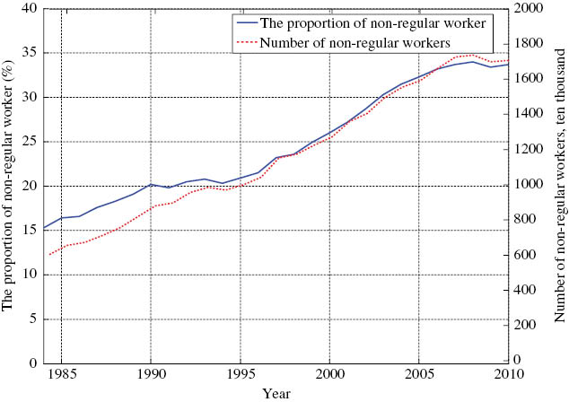
The share and number of non-regular workers.
Note: The solid line indicates the proportion of non-regular workers the total employed workers. The dashed line indicates the number of non-regular workers. Sample covers 1984–2010.
Non-regular workers differ from regular workers in terms of their hiring and separation costs. Labor costs associated with non-regular workers are less than those of regular workers. Japanese employers are not subject to unemployment insurance, pension and health insurance payroll taxes on many non-regular workers. According to OECD (2011), less than half of non-regular workers are included in employee’s pension and health insurance, while less than two-thirds are covered by employment insurance. This is in contrast to virtually complete coverage of regular workers. In addition, compared with regular workers, non-regular workers receive fewer company provided fringe benefits and less firm-provided training (OECD 2011). A government survey found that one of the principle reasons for a business establishment to utilize non-regular employment is to reduce labor costs (MHLW 2008; JILPT 2011).
In Japan, while the employment protection of regular workers is fairly strict, non-regular employment is relatively lightly regulated. According to the employment protection legislation (EPL) indicator complied by OECD (2004) and Venn (2009), Japan’s EPL is stricter for regular employment and is less strict for non-regular employment compared to the OECD average. Furthermore, as Aoyagi and Ganelli (2013) point out, anecdotal evidence suggests that in Japan courts apply stricter standards for dismissals of regular workers compared to non-regular ones.
Figure 2 shows the unemployment rate and its trends. I obtain the data from LFS. In order to obtain the trend component of the data, I use the Hodrick-Prescott filter (Hodrick and Prescott 1997). Following Ball and Mankiw (2002), I consider two different values of the smoothing parameter in the HP filter, λ=100 and λ=1000. The unemployment rate has been significantly low until the middle of 1990s, with an average of 2.5%. It increased gradually and exceeded 5% in 2001. Then, the unemployment rate declined in the early and middle of 2000s, but it increased after the global financial crisis occurred in 2008.
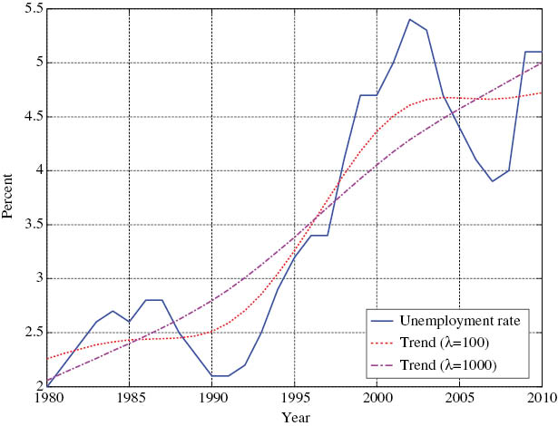
Unemployment rate and trends.
Note: The solid line indicates the unemployment rate. The dashed line indicates the trend of the unemployment rate constructed by using the HP-filter with smoothing parameter 100. The dash-dotted line indicates the trend of the unemployment rate constructed by using the HP-filter with smoothing parameter 1000. Sample covers 1980–2010.
Figure 3 presents the productivity growth rate and its trends. Productivity is measured as real output per employed workers. The output measure is based on the National Income and Product Accounts, while employment is constructed by Statistics Bureau and Statistics Center. The productivity growth rate is the first differenced logged labor productivity. Similar to the unemployment rate, I use the HP filter to obtain the smoothed series of the productivity growth rate. The productivity growth rate increased until the middle of 1980, and then gradually declined. The productivity growth rate declined sharply in 1990s and was relatively stable in 2000s.
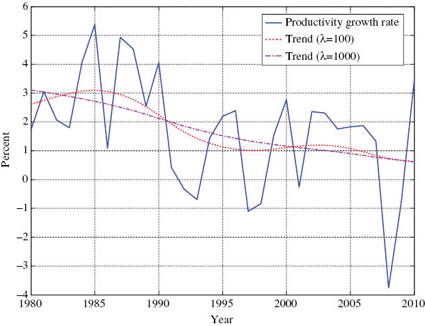
Productivity growth rate and trends.
Note: The solid line indicates the productivity growth rate. Labor productivity is measured as real output per employed workers, and the productivity growth rate is the first differenced logged labor productivity. The dashed line indicates the trend of the productivity growth rate constructed by using the HP-filter with smoothing parameter 100. The dash-dotted line indicates the trend of the productivity growth rate constructed by using the HP-filter with smoothing parameter 1000. Sample covers 1980–2010.
Figure 4 shows smoothed series for the proportion of non-regular workers to total employed workers (φ), the unemployment rate (u), and the productivity growth rate (g). Table 1 summarizes the relationship among smoothed series of these three variables.
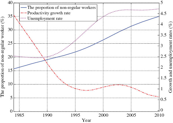
Productivity growth and labor market variables.
Note: The solid line indicates the trend of the proportion of non-regular workers to total employed workers. The dashed line indicates the trend of the productivity growth rate. The dash-dotted line indicates the trend of the unemployment rate. The trends are HP filters with the smoothing parameter 100. Sample covers 1984–2010.
Summary statistics: correlation matrix.
| ϕ | g | u | |
|---|---|---|---|
| φ | 1 | –0.768 | 0.954 |
| g | – | 1 | –0.748 |
| u | – | – | 1 |
Correlation between the proportion of non-regular workers to total employed workers (φ), the productivity growth rate (g), and the unemployment rate (u). All series are smoothed with the Hodrick-Prescott filter with the smoothing parameter λ=100. Sample covers 1984–2010.
Table 1 and Figure 4 show that there is a strong negative relationship between productivity growth and the proportion of non-regular workers to total employed workers in their trend terms. The correlation between these series is –0.768. I also find that the productivity growth rate is negatively correlated with the unemployment rate and the correlation is –0.748. Interestingly, there is a positive relationship between the proportion of non-regular workers to total employed workers and the unemployment rate. The correlation between them is 0.954.
In order to calculate the effect of productivity growth on labor market variables, following previous studies (e.g. Pissarides and Vallanti 2007; Miyamoto and Takahashi 2011), I consider the following linear relationship between the long-run labor market variables and long-run productivity growth
where yt is the long-run labor market variables (the proportion of non-regular workers to total employed workers φ and the unemployment rate u), gt is the long-run productivity growth rate, β0 and β1 are parameters, and εyt is a well-behaved stochastic disturbance. By using the trend components of the productivity growth rate and labor market variables, I have the following OLS estimates:
and
where Newey–West HAC standard errors are reported in parentheses.
Although caution is needed to see the results due to the small sample size, the regressions show that a 1% increase in the long-run productivity growth reduces the proportion of non-regular workers by 4.32%. It is also shown that a 1% increase in the long-run growth reduces the unemployment rate by 0.65%. This is in line with existing empirical studies. For example, Blanchard and Wolfers (2000) estimate that a 1% increase in the growth rate leads to a 0.25%–0.7% increase in the unemployment rate.
3 Model
I consider a continuous time search and matching model with two types of jobs, a regular job and a non-regular job. Regular and non-regular jobs differ in their separation and hiring costs.[7] The difference between the two types of jobs is due to labor laws and institutions that impose different duration, termination and hiring costs on employers.[8] The basic structure of the model follows Pissarides (2000). In order to study the impact of productivity growth on labor market dynamics, I introduce disembodied technological progress, as in Pissarides (2000) and Pissarides and Vallanti (2007).
The environment: There is a large measure of firms and a unit measure of workers in an economy. Both firms and workers are infinitely lived and risk neutral. Each firm can have at most one job. There are two types of jobs: regular (R) and non-regular (N) jobs. A firm must decide ex ante, that is, before searching for a worker, whether it will open a regular or a non-regular job. Regular and non-regular jobs differ in their separation and hiring costs. A regular job is terminated with a low exogenous separation rate δR, in which the firm needs to pay a firing cost ft.[9] A non-regular job is terminated with a high exogenous separation rate δN (δN>δR), in which case the firm does not need to pay the firing cost. Furthermore, it is assumed that the cost of posting a new regular job, γR, is higher than that of posting a non-regular job, γN.
There are two types of workers: regular workers and non-regular workers. They differ in their skill level. It is assumed that a regular worker has higher skill than a non-regular worker. The proportion of regular workers in the economy is denoted by ϕt. I assume that while a non-regular worker cannot change her skill level in the short-run, she can up-grade her skill by paying the cost of training ct and become a regular worker in the long-run.
Production technology: Firms with filled regular jobs and firms with filled non-regular jobs produce two intermediate goods that are then sold in a competitive market and immediately transformed into the final consumption good. Workers derive utility from consumption of the final good and maximize the present discount value of their utility. On other hand, firms maximize the present discount value of their income. Discount rate is denoted by r.
Production of a firm of type j∈{R, N} at time t is given by
where At is a general productivity parameter common to all producing jobs and ejt is employment in type j jobs. Suppose that the leading technology in the economy is driven by an exogenous invention process that grows at the rate g<r. Thus, At=A exp(gt), where A>0 is some initial productivity level.
The technology of production for the final good is given by
where σ<1 and the parameter α is the relative share of the regular job’s input in final production. The elasticity of substitution between yR and yN is 1/(1–σ). The price of final goods is normalized to one. Since the two intermediate goods are sold in competitive markets, their prices are
and
The labor market: The labor market is subject to frictions. Firms and workers cannot meet instantaneously but must go through a time-consuming search process. I assume that the search process is directed. Each firm posts either a vacancy for a regular worker or one for a non-regular worker. Free entry determines endogenously the number of firms in each labor market. On the other hand, unemployed workers search for jobs. Specifically, regular workers direct their search towards the labor market for type R jobs, whereas non-regular workers search for type N jobs. The number of matches between type j vacancies and unemployed workers search for type j jobs is determined by the matching function
where vjt is the number of vacancies posted and ujt is the number of unemployed workers. The matching function ℳ(vjt, ujt) is continuous, twice differentiable, increasing in its arguments, and has constant returns to scale. Define θjt=vjt/utt as labor market tightness in the market for type j jobs. The rate at which a firm with a vacancy is matched with a worker is ℳ(vjt, ujt)/vjt=ℳ(1, ujt/vjt)≡q(θjt). Similarly, the rate at which an unemployed worker is matched with a firm is ℳ(vjt, ujt)/ujt=θjtq(θjt). Since the matching function has constant returns to scale, q(θjt) is decreasing in θjt and θjtq(θjt) is increasing in θjt.
Since the total number of workers in the economy is one, I have
The total unemployed workers are given by ut=uRt+uNt. Since the labor force is one, ut represents an aggregate unemployment rate. The fraction of regular workers in the economy is denoted by ϕ. Then, I have
The evolution of unemployment in the market for type j jobs is given by the difference between the flow into unemployment and flow out of it. Thus,
3.1 The value functions
I restrict my attention to stationary equilibrium, and labor market tightness is assumed to be constant over time. The value of a firm with a type j filled job, Πjt, is characterized by the following Bellman equation:
where wjt is the wage at time t, Vjt is the value of a firm with a type j vacant job and 𝕀R is an indicator function that equals one if j=R and equals to zero otherwise. The firm receives flow revenues PjtAt–wjt, which is the productive output of the match minus the wage paid to the worker. The match is destroyed by the exogenous shock at rate δj, in which case the firm loses its asset value of the filled job, pays the firing tax, and obtains the value of a vacant job. It is important to note that job separation rates are different between type R jobs and type N jobs, and only firms with type R jobs pay the firing cost ft. The asset value of a match is expected to change over time due to exogenous technological progress.
The value of a firm with a type j vacant job at time t is given by
where γjt is the cost of posting a vacancy and
Given the starting wage
I now turn to the worker’s side. The value of an employed worker in a firm with a type j job at time t, Wjt, is characterized by the following Bellman equation:
where Ujt is the value of an unemployed worker who searches for a job of type j. The value of an employed worker is determined by several factors. The worker receives the wage wj. The match may be destroyed by the exogenous shock at rate δj, in which case the worker loses the current asset value and obtains the asset value of being unemployed. The asset value of a match is expected to change over time due to technological progress.
The value of an unemployed worker searching for a job of type j is
where zjt is the unemployment benefits and
Note that an initial value of an employed worker in a type N job is the same to the continuing value of it. Thus,
The firm that has a job with value Πjt at time t expects to make a capital gain of
I focus on the steady state. This corresponds to a balanced growth path where the economy grows at the rate of productivity growth g. To make the model stationary, I assume that all exogenous variables grow at the rate of productivity growth g.[10] Thus, I define six positive exogenous parameters γj, zj, f, and c such that γjt=Atγj, zjt=Atzj, ft=Atf, and ct=Atc.
Replacing the capital gain by its steady-state value, the above Bellman equations can be rewritten as follows:
and
The wages are determined through the Nash bargaining between a firm and a worker over the share of expected future joint income. Let βj∈(0, 1) be the worker’s bargaining power. Due to the firing cost, the wage determination mechanism differs between two markets. I first look at the wage determination in the market for type R jobs. When a firm and a worker first meet, the payoff to the firm is
Once the worker is employed, the firm has to pay the firing tax Af if the firm fails to agree to a continuation wage. Thus, the continuing wage is chosen as
Since a firm with the type N job does not need to pay the firing cost, there is no difference between a starting wage and a continuation wage. The wage in the type N job is determined by
It is assumed that a non-regular worker can upgrade her skill by paying the training cost Ac.[11] In equilibrium, the value of staying in the R sector is equivalent to that of staying in the N sector. Thus, arbitrage by workers between sectors implies that
Free entry implies that the value of a vacant job is zero in equilibrium. Thus,
Finally, the steady-state unemployment is given by
and
3.2 Characterization of steady-state equilibrium
A steady-state equilibrium is a profile
The free entry condition Vj=0 together with (4) yields
By using (9), (13), and (16), the value of an unemployed worker in the j sector can be rewritten as
By using all the value functions (3)–(8), the free entry condition, and the wage sharing rules (9)–(11), I obtain the following equilibrium wages:
and
Making use of (12) and (17), I derive the following equilibrium condition:
The numbers of employed workers in the sector R and N are determined as eR=ϕ–uR and eN=1–ϕ–uN. Then, the aggregate production in the sector R and N are obtained by
Then, the prices of the two inputs can be obtained as
Substituting the price of goods in the R sector and (18) into (5) and using the free entry condition VR=0 and (4), I obtain the equilibrium job creation condition
Similarly, by substituting the price of goods in the N sector and (19) into (3), and using (4) and (13), I have the following job creation condition in the type N job sector:
The job creation condition states that the expected cost of posting a vacancy, the left-hand side of (21)((22)), is equal to the firm’s share of the expected net surplus from a new job match, the right-hand side of (21)((22)).
The system of equations (20), (21), and (22) determine endogenous variables θR, θN, and ϕ. Given θR, θN, and ϕ, equations (14) and (15) determine the number of unemployed workers in the sectors R and N, respectively.
4 Quantitative analysis
In this section, I calculate the equilibrium of the above model using numerical methods. I first calibrate the model to match several dimensions of the Japanese labor market data. Then, I perform quantitative comparative statics by calculating the steady-state response to an increase in the rate of productivity growth. I also discuss the sensitivity of the results to my choice of parameter values.
4.1 Calibration
I choose the model period to be 1-year and set the discount rate at r=0.036. This choice of the parameter is somewhat a priori, but is consistent with other studies such as Braun et al. (2006). Since the level of productivity does not influence the steady-state, I normalize A=1 without loss of generality. For a benchmark case, I set g=0.016, the average productivity growth rate in Japan from 1980 to 2014.
For the final goods production function, I choose σ=0 for the benchmark specification. Thus, the production function is Cobb-Douglas.
The matching function is Cobb-Douglas, given by
Given this, I target the average monthly job finding rate of 0.142 and the average monthly separation rate of 0.0048, which are reported by Miyamoto (2011) and Lin and Miyamoto (2012).[13] The Report on Employment Service conducted by Ministry of Health, Labour and Welfare (MHLW) reports the job openings to applications ratios (yuko kyujin bairitsu) of both regular and temporary workers, which reflects labor market tightness. Based on the dataset, I target the ratio of labor market tightness for non-regular workers to that for regular workers θN/θR=2.24. I also target the share of non-regular workers in total employed workers. Based on the LFS, the mean value of the ratio over the period of 1984–2014 is 0.26. From the Survey on Employment Trends conducted by MHLW, the ratio of the job-finding rate for regular workers to that for non-regular workers is 0.45 and the ratio of the separation rate for regular workers to that for non-regular workers is 0.49. I target these ratios.
Following Esteban-Pretel, Nakajima, and Tanaka (2011), I target the unemployment flow utility zj to be 40% of the average wage in each sector.[14] I also target a wage ratio between regular workers and non-regular workers to be equal to 0.6, based on the Basic Survey on Wage Structure conducted by MHLW. Finally, following Nosaka (2011), I target the firing cost f to be approximately 0.5 of an average wage.[15] Without loss of generality, I normalize θR to one.
I thus have 11 target moments and 11 model parameters: c, f, zR, zN, α, mR, mN, δR, δN, γR, and γN. I choose the parameter values that most closely match the 11 target moments. The parameter values are summarized in Table 2.
Parameter values.
| Parameter | Description | Value | Source/target | |
|---|---|---|---|---|
| A | A general productivity parameter | 1.0 | Normalization | |
| r | Discount rate | 0.036 | Data | |
| g | The rate of productivity growth | 0.016 | Data | |
| ξ | Elasticity of matching function | 0.6 | Lin and Miyamoto (2014) | |
| βR | Worker’s bargaining power in the R sector | 0.5 | Symmetric Nash bargaining | |
| βN | Worker’s bargaining power in the N sector | 0.5 | Symmetric Nash bargaining | |
| σ | CES-elasticity parameter | 0.0 | Cobb-Douglas | |
| c | Cost of being a regular worker | 12.33 |  | Match target moments: |
| f | Firing cost | 0.334 | Job finding rate | |
| zR | Flow value of unemployment in the R sector | 0.267 | Separation rate | |
| zN | Flow value of unemployment in the N sector | 0.160 | Replacement rate | |
| α | CES-weight | 0.828 | Share of non-reg.employed workers | |
| mR | Scale parameter of matching function in the R sector | 1.316 | Job find. rate for R workers/job find. rate for N workers | |
| mN | Scale parameter of matching function in the N sector | 2.118 | Sep. rate for R workers/sep. rate for N workers | |
| δR | Separation rate in the R sector | 0.046 | Wage for N workers/wage for R workers | |
| δN | Separation rate in the N sector | 0.092 | Tightness for N workers/tightness for R workers | |
| γR | Vacancy cost in the R sector | 0.371 | Ratio of firing cost to wage | |
| γN | Vacancy cost in the N sector | 0.103 | Normalization |
Selected model solutions under the calibrated parameter values are reported in Table 3. The unemployment and job finding rates in the economy, the ratio of non-regular workers to total employed workers, and the ratios of labor market tightness and job-finding rates between sectors are equal to their target values. Unemployment in the regular-job sector, 0.025, is much higher than that in the non-regular job sector, 0.008. The number of vacancies in the regular job sector is 0.025, while that in the non-regular job sector is 0.018. Prices in the regular job sector are about 69% higher than those in the non-regular job sector.
Model solutions.
| Variable | Description | Solution |
|---|---|---|
| θR | Labor market tightness in the R sector | 1.0 |
| θN | Labor market tightness in the N sector | 2.24 |
| ϕ | The proportion of non-regular employed workers | 0.26 |
| uR | Unemployment in the R sector | 0.025 |
| uN | Unemployment in the N sector | 0.008 |
| u | Total unemployment | 0.033 |
| vR | Vacancies in the R sector | 0.025 |
| vN | Vacancies in the N sector | 0.018 |
| eR | Employment in the R sector | 0.716 |
| eN | Employment in the N sector | 0.252 |
| e | Total employment | 0.968 |
| θRq(θR) | Job finding rate in the R sector | 1.316 |
| θNq(θN) | Job finding rate in the N sector | 2.924 |
| wR | Wage in the R sector | 0.668 |
| wN | Wage in the N sector | 0.401 |
| PR | Price in the R sector | 0.691 |
| PN | Price in the N sector | 0.410 |
4.2 Effects of growth on the labor market
I now examine the effects of productivity growth on labor market variables of interest by calculating the steady-state response to an increase in the productivity growth rate g. The results are shown in Figure 5.
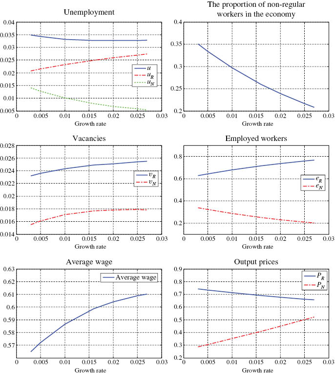
Comparative statics for the productivity growth rate g.
A faster rate of productivity growth increases regular employed workers and reduces non-regular employed workers, lowering the proportion of non-regular workers in the economy. The negative relationship between productivity growth and the share of non-regular workers is consistent with the empirical finding in Section 2. The channel through which faster productivity growth reduces the share of non-regular workers is as follows. Since an increase in productivity growth makes to work in the regular sector more appealing by reducing costs of working in the regular sector, a larger number of job seekers shifts from the non-regular sector to the regular sector. This increases job creation in the regular sector and thus regular employed workers.
Under my choice of parameter values, faster productivity growth reduces the aggregate unemployment rate, which is also consistent with the data. In order to understand the mechanism behind the effect of productivity growth on unemployment, it is useful to see the effect of productivity growth on vacancies.
The impact of productivity growth on vacancies is ambiguous because there are several counteracting effects. First, a rise in the productivity growth rate increases vacancies in both sectors. Since a higher rate of productivity growth increases the return from creating a job, firms in both sectors have a greater incentive to open vacancies. This is because the cost of creating a vacancy is paid at the start but the profits accrue in the future. When the growth rate rises, all future income flows are discounted at lower rate, so firms are encouraged to create more vacancies. This effect is well-known as the capitalization effect. Second, faster productivity growth tends to increase vacancy creation in the regular job sector but to reduce vacancy creation in the non-regular sector through increasing worker flows from the non-regular job sector to the regular job sector. An increase in worker flows from the non-regular job sector to the regular job sector makes firms in the regular sector find a worker easier and induces more vacancy creation. On the other hand, in the non-regular job sector, since a number of job seekers decreases due to the worker reallocation, firms have less intensive to open vacancies. I call this the worker reallocation effect. Third, faster productivity growth affects output prices and thus vacancy creation in both sectors. An increase in the productivity growth rate reduces the output price in the regular job sector and increases the output price in the non-regular job sector. An increased employment in the regular sector increases the supply of output, lowering the price of goods, while a decreased employment in the non-regular job sector reduces output and thus increases the price of goods. This price effect reduces vacancy creation in the regular job sector by reducing the return from creating a job, while it increase vacancy creation in the non-regular job sector by increasing the return from creating a job.
As seen in Figure 5, under calibrated parameter values, faster productivity growth increases vacancies in both sectors. In the regular job sector, since the capitalization and worker reallocation effects dominate the price effect, faster productivity growth increases vacancies. In the non-regular job sector, the capitalization and price effects dominate the worker reallocation effect. As a result, the increase in productivity growth leads to more vacancies.
I now turn to see the effect of productivity growth on unemployment. Since in the non-regular job sector, firms open more vacancies and a number of job seeker decreases due to the worker reallocation effect, the job-finding rate increases. This leads to a lower unemployment rate in the non-regular job sector. On the other hand, in the regular job sector, increased worker flows from the non-regular job sector cause congestion to one another when trying to match with vacancies. Although firms post more vacancies, the congestion effect is strong enough to reduce the job-finding rate and thus increase the unemployment rate.
While faster productivity growth increases the unemployment rate in the regular job sector, it reduces the unemployment rate in the non-regular job sector. Thus, the effect of faster productivity growth on the aggregate unemployment rate depends on which effect dominates. Under my choice of parameter values, since the latter effect dominates the former one, faster productivity growth reduces the aggregate unemployment rate.
Figure 5 shows that faster productivity growth increases the average wage in the economy. This is because faster productivity growth increases the share of regular employed workers whose wages are higher than non-regular employed workers’ wages.
Finally, I study whether the model’s prediction on the response of the proportion of non-regular jobs in the economy to productivity growth is empirically plausible. In Section 2, I find that a 1% increase in the productivity growth rate reduces the proportion of non-regular workers by 4.32%. In my model, a 1% increase in the growth rate reduces the proportion of non-regular workers by 5.8%. Thus, my model can explain the observed response of non-regular workers to growth.
4.3 Sensitivity analysis
In the benchmark case, faster productivity growth reduces the proportion of non-regular workers and the aggregate unemployment rate. I now discuss how these results vary with the value of the firing cost f and the parameter in the final goods production function σ. When I change these parameters, I also re-calibrate parameters c, zR, zN, α, mR, mN, δR, δN, γR, and γN in order to maintain my calibration target values.
First, I consider the impact of the value of the firing cost f. Figure 6 shows the relationship between the productivity growth rate and the aggregate unemployment rate. It also shows the relationship between the productivity growth rate and the proportion of non-regular workers in the economy for different values of the firing cost f. Although the size of impact is slightly changed, the sign of the relationship between growth and unemployment does not change. It is also clear that allowing for firing costs f to vary does not have a significant impact on the relationship between the rate of productivity growth and the proportion of non-regular workers.
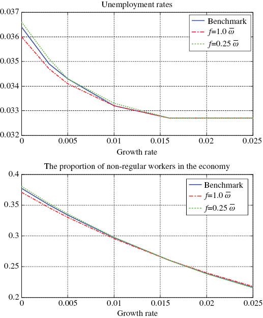
Sensitivity analysis with respect to f.
Next, I discuss the sensitivity of the results to my choice of the parameter value σ. In my benchmark calibration, I set σ=0 and assume that the final goods production function is Cobb-Douglus. I now consider two different values of σ, –1 and –1/3. In the former case, the elasticity of substitution is 0.5 and in the latter case, the elasticity of substitution is 0.75. Figure 7 shows the results. It shows that the negative relationship between growth and unemployment is robust to change in values of σ. Figure 7 also shows that the negative relationship between growth and the share of non-regular employment is robust to choice of parameter values of σ, decreases.
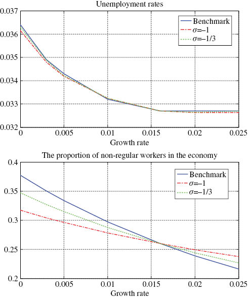
Sensitivity analysis with respect to σ.
5 Discussion
In this section, I first study the welfare properties of equilibrium. I then discuss the role of job separation when the effect of productivity growth on the labor market variables is examined.
5.1 Welfare analysis
I now analyze the welfare properties of equilibrium. In order to consider the efficient allocation in this economy, I analyze the social planner’s problem. The social welfare function used by the social planner is given by
Welfare is equal to the total flow of output, plus the unemployment benefits, minus the flow vacancy cost incurred in both sectors and the firing cost.[16] Note that this welfare function does not take account of distributional considerations.
The social planner is subject to the same matching constraints as firms and workers. Thus, the social planner’s problem is to maximize (23) subject to (1). The first-order conditions of this problem yield the following equation that determine the socially efficient θj.
where η(θj) is the negative of the elasticity of q(θj), and it is a number between 0 and 1.
By comparing this equation with the decentralized equilibrium conditions (21) and (22), we can see that the decentralized equilibrium is efficient if and only if βj=η(θj). This is the standard Hosios condition for efficiency. When βj>η(θj), there will be too little job creation, and the composition of jobs will be biased toward non-regular jobs. Thus, if βj=η(θj) holds in both sectors, total number of jobs is efficient and the job composition is also efficient in the decentralized equilibrium. This result is in contrast to the random search model in which there is always an inefficient job composition [see Acemoglu (2001)].
It is important to note that for any value of the firing cost f, the above-mentioned result holds. This is because the firing cost is taken into account when wages are negotiated. However, this is not the case for the training cost c. So far, I have imposed the condition that c=0 when I considered the social planner’s problem and demonstrated that we need the Hosis condition to restore efficiency. However, when c has a positive value, the Hosios condition does not restore efficiency. This is because the training cost is sunk at the wage determination stages.
5.2 Endogenous job separation
In the present model, the job destruction process is exogenous and all the changes in job match characteristics are coming from the endogenous job creation dynamics. However, productivity growth may affect employment and worker flows via job separation. Indeed, productivity growth reduces job separation and lowers unemployment in the US (See Miyamoto and Takahashi 2011). This section discusses the role of endogenous job separation.
First, I examine a long-run relationship between productivity growth and the separation rate in Japan. Following Miyamoto (2011) and Lin and Miyamoto (2012), I construct the series of the separation rate from the LFS. By applying the same method in Section 2 to this time series, I find that there is a negative relationship between productivity growth and the separation rate (See Figure 8). Their correlation is –0.83. This suggests that in order to study the impact of growth unemployment, it is better to use a model in which job separation is endogenously determined.
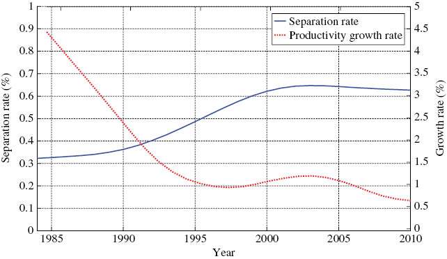
Productivity growth and separation rates.
Note: The solid line indicates the trend of the separation rate. The dashed line indicates the trend of the productivity growth rate. The trends are HP filters with the smoothing parameter 100. Sample covers 1984–2010.
I now develop a version of my model in which job separation is endogenously determined. The details of the model are presented in Appendix. Similar to Section 4.2, I examine the effects of productivity growth on labor market variables of interest by calculating the steady-state response to a change in the productivity growth rate g. The results are summarized in Table 4.
Reults of the endogenous separation model.
| Growth rate | Unemployment | The proportion of non-regular workers | Separation rate (monthly, %) | ||||
|---|---|---|---|---|---|---|---|
| Total | R-sector | N-sector | Total | R-sector | N-sector | ||
| 0.014 | 0.083 | 0.028 | 0.056 | 0.281 | 1.76 | 0.47 | 5.07 |
| 0.015 | 0.058 | 0.027 | 0.031 | 0.271 | 1.11 | 0.43 | 2.93 |
| 0.016 | 0.033 | 0.025 | 0.008 | 0.260 | 0.48 | 0.38 | 0.77 |
| 0.017 | 0.031 | 0.027 | 0.003 | 0.269 | 0.39 | 0.42 | 0.31 |
| 0.018 | 0.034 | 0.031 | 0.003 | 0.279 | 0.48 | 0.48 | 0.31 |
The effects of productivity growth on the labor market variables in the model with endogenous separation are different from those in the benchmark model (the model without endogenous separation). In the benchmark model, under plausible parameter values, faster productivity growth reduces unemployment and the proportion of non-regular workers. In contrast, the endogenous separation model shows that the U-shaped relationship between productivity growth and the unemployment rate (the proportion of the non-regular workers). Thus, when productivity growth is low, faster productivity growth reduces unemployment and the proportion of non-regular workers. On the other hand, when productivity growth is high, an increase in the productivity growth rate increase these two variable. This model’s prediction is counterfactual to what observed in data. Furthermore, the model shows the U-shaped relationship between productivity growth and the aggregate separation rate, which is also inconsistent with the above mentioned empirical finding.
The key to understand this result is the so-called outside option effect identified by Prat (2007). Prat (2007) demonstrates that, in the search and matching model with endogenous job separation, faster productivity growth is more likely to increase job separation by increasing workers’ outside option; consequently, the model can generate a positive relationship between productivity growth and unemployment.[17] In my endogenous job separation model, when productivity growth is low, the worker reallocation effect mitigates the outside option effect. Therefore, faster productivity growth reduces the proportion of non-regular workers and the separation rate. On the other hand, when productivity growth is high, the worker reallocation effect weakens and thus faster productivity growth increases job separation and unemployment.
6 Conclusion
This paper studies an effect of productivity growth on both non-regular employment and unemployment. I document the fact that productivity growth reduces both the share of non-regular employment in the economy and the unemployment rate at low frequencies in Japan. To account for these empirical findings, I develop a search and matching model with disembodied technological progress and two types of jobs, regular and non-regular jobs. The numerical analysis demonstrates that under the set of plausible parameter values, faster growth reduces the proportion of non-regular workers and the unemployment rate. Thus, my model succeeds to capture the empirical pattern of the share of non-regular employment and the unemployment rate in response to productivity growth.
A number of important issues remain for future research. Considering an intensive margin for adjusting labor input is an important issue. It is shown that in Japan, the labor input adjustment relies on both working hour adjustment and changing the number of workers.[18] One would expect that an increase in non-regular workers shifts the burden of adjustment from hours to employment. Thus, the increase in non-regular workers affects both intensive and extensive margins for adjustment labor input. Another important line of future research is to consider a link between the labor and the goods markets and their impact on the regular and non-regular employment. In my model, the interaction between the product and the labor market markets is simple. A regular and non-regular sector produces intermediate goods that are used to produce the final good. The aggregate production function introduces a link between labor market conditions in the two sectors through prices of the intermediate goods. To develop a model in which the interaction between product market structure and labor market outcomes is scrutiny and study an effect of productivity growth on non-regular employment and unemployment is a fruitful avenue for research.
Acknowledgments:
I am grateful to the editor Tiago Cavalcanti and an anonymous referee for very helpful comments and suggestions. I also thank Ryoichi Imai, Makoto Kakinaka, Koji Kotani, Noritaka Kudoh, Masaru Sasaki, Makoto Yano and seminar participants at WEAI 10th Biennial Pacific Rim Conference at Keio University and Search Theory Workshop at Osaka University for their helpful comments. All remaining errors are mine. Part of this research is supported by the Grants-in-Aid for Young Scientists of the Japan Society for the Promotion of Science (Kakenhi No. 24730179) and IUJ Research Institute research fund.
Appendix
This appendix presents a version of my model in which job separation is endogenously determined. The basic structure of the model is the same to that of my original model. While matches are terminated for an exogenous reason in my original model, I now assume that match separation occurs due to both exogenous and endogenous reasons. I use the same notations as in my original model.
Let the output of each firm in the sector j is now given by pjAxj, where xj is match-specific idiosyncratic productivity. It is assumed that xj=1 when a job is created. A randomly selected fraction δj of jobs break up for exogenous reasons and another randomly selected fraction λj receives a productivity shock that changes each job’s idiosyncratic productivity xj to some other value
The value functions of firms and workers are given by
The wages are determined through the Nash bargaining between a firm and a worker over the share of expected future joint income. Thus, the starting and continuation wages are determined by the following equations:
When an idiosyncratic shock arrives, the firm can either continue to produce or close the job down. The optimal decision of the firm is to continue its production if
Free entry condition is
The arbitrage by workers between sectors implies that
The steady-state unemployment is given by
The technology of production for the final good is given by
where yjt is output in the sector j and the parameter α is the relative share of the regular job’s input in final production. The elasticity of substitution between yR and yN is 1/(1–σ) where σ<1. The price of final goods is normalized to one. Since the two intermediate goods are sold in competitive markets, their prices are
and
Calibration: The basic parameter values are the same to those of the original model. Following Silva and Toledo (2009), I assume that endogenous job separation accounts for, on average, 35% or total separations. Following Mortensen and Pissarides (1994), I assume that the idiosyncratic productivity distribution G is uniform in the range [0,1]. Furthermore, I assume that δR=δN. The parameters c, f, zj, α, mj, δj, γj and λj are calibrated by using original model’s targets.
References
Acemoglu, D. 2001. “Good Jobs versus Bad Jobs.” Journal of Labor Economics 19: 1–21.10.1086/209978Search in Google Scholar
Albrecht, J. W., L. Navarro, and S. B. Vroman. 2009. “The Effects of Labor Market Policies in an Economy with an Informal Sector.” Economic Journal 119: 1105–1129.10.2139/ssrn.905539Search in Google Scholar
Alonso-Borrego, C., J. Fernández-Villaverde, and J. E. Galdón-Sánchez. 2005. “Evaluating Labor Market Reforms: A General Equilibrium Approach.” NBER Working Papers 11519, National Bureau of Economic Research, Inc.10.3386/w11519Search in Google Scholar
Amaral, P. S., and E. Quintin. 2006. “A Competitive Model of the Informal Sector.” Journal of Monetary Economics 53: 1541–1553.10.1016/j.jmoneco.2005.07.016Search in Google Scholar
Antunes, A. R., and T. V. Cavalcanti. 2007. “Start up Costs, Limited Enforcement, and the Hidden Economy.” European Economic Review 51: 203–224.10.1016/j.euroecorev.2005.11.008Search in Google Scholar
Aoyagi, C., and G. Ganelli. 2013. “The Path to Higher Growth: Does Revamping Japan’s Dual Labor Market Matter?” IMF Working Paper WP/13/202.10.5089/9781484391303.001Search in Google Scholar
Asano, H., T. Ito, and D. Kawaguchi. 2013. “Why has the Fraction of Nonstandard Workers Increased? A Case Study of Japan.” Scottish Journal of Political Economy 60: 360–389.10.1111/sjpe.12015Search in Google Scholar
Ball, L., and N. G. Mankiw. 2002. “The NAIRU in Theory and Practice.” Journal of Economic Perspectives 16: 115–136.10.3386/w8940Search in Google Scholar
Bentolila, S., and G. Saint-Paul. 1992. “The Macroeconomic Impact of Flexible Labor Contracts, with an Application to Spain.” European Economic Review 36: 1013–1047.10.1016/0014-2921(92)90043-VSearch in Google Scholar
Blanchard, O. J., and J. Wolfers. 2000. “The Role of Shocks and Institutions in the Rise of European Unemployment: The Aggregate Evidence.” Economic Journal 110: 1–33.10.3386/w7282Search in Google Scholar
Braun, R. A., J. Esteban-Pretel, T. Okada, and N. Sudou. 2006. “A Comparison of the Japanese and US Business Cycles.” Japan and the World Economy 18: 441–463.10.1016/j.japwor.2006.03.002Search in Google Scholar
Esteban-Pretel, J., R. Nakajima, and R. Tanaka. 2010. Japan’s Labor Market Cyclicality and the Volatility Puzzle. Graduate Institute for Policy Studies, Mimeo.Search in Google Scholar
Esteban-Pretel, J., R. Nakajima, and R. Tanaka. 2011. “Are Contingent Jobs Dead Ends or Stepping Stones to Regular Jobs? Evidence from a Structural Estimation.” Labour Economics 18: 513–526.10.1016/j.labeco.2010.12.010Search in Google Scholar
Genda, Y., A. Hijzen, R. Kambayashi, and H. Teruyama. 2012. Labour Input Adjustment in Japan. Mimeo.Search in Google Scholar
Hodrick, R. J., and E. C. Prescott. 1997. “Postwar US Business Cycles: An Empirical Investigation.” Journal of Money, Credit, and Banking 29: 1–16.10.2307/2953682Search in Google Scholar
Hopenhayn, H., and R. Rogerson. 1993. “Job Turnover and Policy Evaluation: A General Equilibrium Analysis.” Journal of Political Economy 101: 915–938.10.1086/261909Search in Google Scholar
Hosios, A. 1990. “On the Efficiency of Matching and Related Models of Search and Unemployment.” Review of Economic Studies 57: 279–298.10.2307/2297382Search in Google Scholar
Japan Institute for Labour Policy and Training (JILPT). 2011. Non-regular Employment–Issues and Challenges Common to the Major Developed Countries. JILPT Report No. 10.Search in Google Scholar
Kudoh, N., H. Miyamoto, and M. Sasaki. 2014. “Employment and Hours over the Business Cycle in a Model with Search Frictions.” IZA Discussion Paper No. 8946.Search in Google Scholar
Lin, C.-Y., and H. Miyamoto. 2012. “Gross Worker Flows and Unemployment Dynamics in Japan.” Journal of The Japanese and International Economies 26 (1): 44–61.10.1016/j.jjie.2011.09.004Search in Google Scholar
Lin, C.-Y., and H. Miyamoto. 2014. “An Estimated Search and Matching Model of the Japanese Labor Market.” Journal of the Japanese and International Economies 32: 86–104.10.1016/j.jjie.2014.03.001Search in Google Scholar
Ministry of Health, Labour and Welfare (MHLW). 2008. General Survey of Diversified Types of Employment, 2007, Tokyo (in Japanese).Search in Google Scholar
Miyamoto, H. 2011. “Cyclical Behavior of Unemployment and job Vacancies in Japan.” Japan and the World Economy 23: 214–225.10.1016/j.japwor.2011.04.001Search in Google Scholar
Miyamoto, H., and Y. Takahashi. 2011. “Productivity Growth, on-the-Job Search, and Unemployment.” Journal of Monetary Economics 58: 666–680.10.1016/j.jmoneco.2011.11.007Search in Google Scholar
Mortensen, D. T., and C. A. Pissarides. 1994. “Job Creation and Job Destruction in the Theory of Unemployment.” Review of Economic Studies 61: 397–415.10.2307/2297896Search in Google Scholar
Mortensen, D. T., and C. A. Pissarides. 1998. “Technological Progress, Job Creation, and job destruction.” Review of Economic Dynamics 1: 733–753.10.1006/redy.1998.0030Search in Google Scholar
Mortensen, D. T., and C. A. Pissarides. 1999. “Job reallocation and Employment Fluctuations. In: Handbook of Macroeconomics, edited by M. Woodford and J. B. Taylor, 1171–1227. vol. 1. Amsterdam: Elsevier Science.10.1016/S1574-0048(99)10026-0Search in Google Scholar
Nosaka, H. 2011. “Business Cycles and Employment by Employment Types in a Job Search Model.” The Economic Review of Kansai University 60: 25–45.Search in Google Scholar
OECD. 2002. OECD Employment Outlook 2002: Paris.Search in Google Scholar
OECD. 2004. Employment Outlook 2004: Paris.Search in Google Scholar
OECD. 2011. OECD Economic Surveys Japan: Paris.Search in Google Scholar
Petrongolo, B., and C. Pissarides. 2001. “Looking Into the Black Box: A Survey of the Matching Function.” Journal of Economic Literature 39: 390–431.10.1257/jel.39.2.390Search in Google Scholar
Pissarides, C. A. 2000. Equilibrium Unemployment Theory, 2nd ed. Cambridge, MA: MIT Press.Search in Google Scholar
Pissarides, C. A., and G. Vallanti. 2007. “The Impact of TFP Growth on Steady-State Unemployment.” International Economic Review 48: 607–640.10.1111/j.1468-2354.2007.00439.xSearch in Google Scholar
Prat, J. 2007. “The Impact of Disembodied Technological Progress on Unemployment.” Review of Economic Dynamics 10: 106–125.10.1016/j.red.2006.09.003Search in Google Scholar
Rebick, M. 2005. The Japanese Employment System: Adapting to a New Economic Environment. Oxford and New York: Oxford University Press.10.1093/0199247242.001.0001Search in Google Scholar
Silva, J. I., and M. Toledo. 2009. “Labor Turnover Costs and the Cyclical Behavior of Vacancies and Unemployment.” Macroeconomic Dynamics 13: 76–96.10.1017/S1365100509080122Search in Google Scholar
Ulyssea, G. 2010. “Regulation of Entry, Labor Market Institutions and the Informal Sector.” Journal of Development Economics 91: 87–99.10.1016/j.jdeveco.2009.07.001Search in Google Scholar
Venn, D. 2009. “Legislation, Collective Bargaining and Enforcement: Updating the OECD Employment Protection Indicators.” www.oecd.org/els/workingpapers.Search in Google Scholar
Wasmer, E. 1999. “Competition for Jobs in a Growing Economy and the Emergence of Dualism.” Economic Journal 109: 349–371.10.1111/1468-0297.00452Search in Google Scholar
©2016 by De Gruyter
Articles in the same Issue
- Frontmatter
- Advances
- Sustainable monetary policy and inflation expectations
- Contributions
- Monetary policy and news shocks: are Taylor rules forward-looking?
- How do firms adjust production factors to the cycle?
- Does fiscal policy affect interest rates? Evidence from a factor-augmented panel
- Advances
- Public provision of health insurance and welfare
- Contributions
- Reallocation effects of recessions and financial crises: an industry-level analysis
- Growth and non-regular employment
- Knowledge licensing in a model of R&D-driven endogenous growth
- The Taylor principle is valid under wage stickiness
- Testing monetary policy optimality using volatility outcomes: a novel approach