Application of stochastic model predictive control for building energy systems using latent force models
-
Thore Wietzke
 ,
Daniel Landgraf
,
Daniel Landgraf

Abstract
The model-based control of building energy systems (BES) is a hard task, since the system identification is very labor-intensive. This results in inexact models, which are subject to parameter uncertainties. Additionally, disturbances like solar radiation have a great impact on the system dynamics. In this paper we used stochastic model predictive control (SMPC) to account for parameter and disturbance uncertainties. The disturbances are modeled as time-dependent Gaussian Processes (GP), which are known as Latent-Force Models (LFM). The proposed approach is evaluated for two different BES using experimentally obtained data. The results show that the LFM-SMPC results in the lowest discomfort with a reasonable higher energy consumption compared to a constant disturbance prediction.
Zusammenfassung
Die modellbasierte Regelung von Gebäudeenergiesystemen (BES) ist eine anspruchsvolle Aufgabe, da die Systemidentifikation sehr arbeitsintensiv ist. Dies führt zu ungenauen Modellen, die mit Parameterunsicherheiten behaftet sind. Außerdem haben Störungen, wie die Sonneneinstrahlung, einen großen Einfluss auf die Systemdynamik. In dieser Arbeit wird eine stochastische modellprädiktive Regelung (SMPC) verwendet, um die Unsicherheiten der Parameter und Störungen zu berücksichtigen. Die Störungen werden als zeitabhängige Gaußprozesse (GP) modelliert, die als Latente-Kraft Modelle (LFM) bezeichnet werden. Der vorgeschlagene Ansatz wird für zwei verschiedene BES anhand experimentell gewonnener Daten bewertet. Die Ergebnisse zeigen, dass das LFM-SMPC im Vergleich zu einer konstanten Störungsvorhersage zu einem geringeren Diskomfort bei einem angemessen höheren Energieverbrauch führt.
1 Introduction
Buildings are responsible for approximately 30 % of global energy consumption [1], with a significant portion dedicated to Heating, Ventilation, and Air Conditioning (HVAC) to maintain occupant thermal comfort. In building energy systems (BES), rule-based controllers (RB) [2] are predominantly used to set the demand and supply points. These controllers often lack insight into the dynamic behavior of the BES, limiting their ability to leverage thermal dynamics for efficient control. Additionally, HVAC systems are frequently oversized to ensure occupant comfort [3]. Consequently, predictive control strategies have significant potential to lower energy consumption. However, maintaining thermal comfort is essential, which can counteract energy efficiency since energy is required to adjust indoor temperatures.
A widely researched alternative to RB control is model predictive control (MPC). It iteratively solves an optimal control problem (OCP) over a time horizon, predicting future states using a model of the system dynamics, while accounting for constraints and disturbances. Using an accurate model is crucial for the control performance but the identification of the system dynamics is a major problem for BES [4]. Additionally, uncertainties in the disturbances, the model parameters and the structure arise, e.g. the number of states or the functional form of the heat transfer between rooms. A promising approach to accurately capture these uncertainties is stochastic model predictive control (SMPC). Disturbances like solar radiation or ambient temperature have a great impact on the temperature inside the building. Thus, including predictions for such disturbances is crucial for the performance of the MPC. These predictions can either be retrieved from local weather forecasting services or have to be made with on-site measurements.
A suitable approach for predicting such disturbances are Latent Force Models (LFM) [5], which are based on Gaussian Processes (GP), so an uncertainty quantification is available [6]. Their main advantage is the state-space reformulation of the underlying GP, leveraging a linear time-complexity for predictions via the Kalman Filter [7]. LFMs have been applied as data-driven approach for disturbance models, which are crucial for model-based control. In [8] a LQR approach was used to control a mass-spring-damper system and showed superior performance, if an LFM was used. The extension to linear SMPC was proposed in [9] which additionally considered input and state constraints. Since many systems are nonlinear in nature [10], showed the application to nonlinear MPC with a better performance of the LFM. In [11] an LFM in combination with MPC was used to predict the occupancy and to control the BES. Another direction without LFMs but with linear SMPC was used in [12] and showed superior performance of the SMPC.
The novelty of this work is the application of nonlinear SMPC and Latent Force Models to BES. To this end, two BES models are used for evaluation: a baseline parametric model with known parameters and a second model developed in EnergyPlus [13], a white-box modeling software. The LFM is used to predict the solar radiation which is one of the major disturbances in BES. Finally, the models are compared based on their levels of constraint violation and energy consumption.
The paper is structured as follows. Section 2 outlines the state-space representation of LFMs and SMPC for nonlinear systems. Section 3 describes the concepts and models of BES and the modeling of solar radiation. In Section 4, the application of SMPC to BES using LFMs is evaluated. Sections 5 concludes the paper and provides an outlook on future work.
2 LFM-based stochastic model predictive control
LFMs are combinations of first-principle models and GPs, where the latter are used as data-based models for unknown parts of the system dynamics. The posterior distribution of the GPs could be inferred by Gaussian process regression, but the required computational effort increases cubically with the number of data points [14]. An alternative approach is to transform the GP prior to a linear state-space model, which allows to apply the Kalman filter equations for state estimation, which is outlined in Section 2.1. The variance of the GPs introduces uncertainty to the system that must be considered by the controller. A suitable control method for stochastic systems is SMPC, which is described in Section 2.2.
2.1 State-space transformation of latent force models
Consider the continuous-time stochastic system
with state
with a mean function m i (t) and a kernel k i (t, t′). In the following, m i (t) = 0 is assumed without loss of generality [6].
GPs are not suitable for the control of systems with short sampling times due to the large computational effort. Therefore, an alternative approach is proposed in [7], where the GPs are reformulated as linear state-space models, for which the state can be estimated using the Kalman filter. In contrast to Gaussian Processes, the iterative procedure of the Kalman filter does not require saving large data sets and the computation time is time-independent. Provided that the spectral density of the kernel is of the form
the i-th element of the disturbance vector (2) can be modeled by the system [7]
with an internal state
A class of kernels that satisfies condition (3) is the Matérn kernel
with δ = |t − t′|, hyperparameters
with hyperparameters
with Kronecker product ⊗, identity matrix I , and number of internal states n M and n P , respectively [15]. If multiple disturbances affect system (1), each GP (2) can be modeled by a linear time invariant system (4), which can be combined to the extended system
where
2.2 Stochastic model predictive control
The system dynamics (1) involve Wiener processes and Gaussian Processes that cause uncertainty. Further uncertainty is introduced, if the states of the system cannot be measured directly but must be estimated. By combining the system dynamics (1) and the disturbance dynamics (8) to an extended system, the system state
x
and the disturbance state
z
can be estimated together, for example using the unscented Kalman filter [16]. Furthermore, a model predictive controller requires predicted trajectories of the disturbance. Since (8) is independent of
x
and
u
, the mean of the disturbance state
where the initial mean and covariance are given by the state estimator. These can be used to calculate the mean of the disturbance
The estimated state, the predicted disturbance and the system model (1) can be utilized to construct a stochastic model predictive controller that solves an optimal control problem (OCP) in every time step. Since x is a random variable, constraints are formulated as chance constraints that must be fulfilled with a certain probability. Therefore, the stochastic OCP
is considered with terminal cost function V, integral cost function l, prediction horizon T, chance constraints h i with probabilities α i , and terminal chance constraints h T,j with probabilities α T,j . An exemplary control loop is shown in Figure 1. Here, the Observer estimates the mean and covariance of the states x and the internal states z . The disturbance prediction is computed by the Disturbance predictor via (9) and (10).
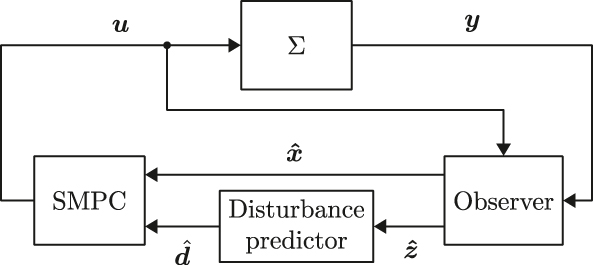
Exemplary control loop for the LFM-SMPC. The observer provides state estimates for the mechanistic model and the latent states, which are used to compute the estimated disturbance trajectory
Solving the stochastic OCP (11) requires the propagation of the uncertain state x through the potentially nonlinear system dynamics function f . The temporal change of the probability density function of x can be represented by a partial differential equation known as the Fokker-Plank equation [17]. Since solving this equation is difficult for general functions f , several methods, such as the unscented transformation, Gaussian quadrature, and polynomial chaos expansion, have been proposed that approximate the solution of the Fokker-Plank equation. For example, the unscented transformation uses sigma-points to capture the uncertainty. They are computed with
where μ x and Σ x denote the mean and covariance of the state x . The additional parameters α UT and κ specify the spread of the sigma points. To recompute the mean and covariance, the unscented transformation uses weights which are applied to the sigma points. These weights are obtained via
with the additional parameter β. Additional information about these methods can be found in [18].
Overall, tracking the covariance for the stochastic OCP results at least in a computational demand of
where z(α i ) and z(α T,j ) are coefficients that can be chosen according to Chebyshev’s inequality [19].
3 Building energy systems
Building Energy Systems are complex systems which consist of a demand and producer side. The producers are Heating, Ventilation and Air Conditioning (HVAC) equipment which provide e.g. cold air and warm water. The demand side consists of thermal zones, which represent areas of similar thermal properties and disturbance influence. For example, the rooms at the south side of a building would be grouped as one thermal zone. A popular approach to modeling dynamic heat transfer is the use of RC thermal networks (see, e.g. [20], [21], [22]).
In this work, only the demand side is considered. The used RC-model for one thermal zone is given in Figure 2. The temperatures of the zone, the exterior wall, the radiator, the neighbor zones and the ambient temperature are denoted as T z , T w , T r , T i and T a , respectively. Additional heat sources like solar radiation or from the HVAC-equipment are omitted in the network for a better overview. The resulting dynamics are given by
with the ventilation heat gain
and the hot water heat flow
where c
∗ are the specific heat capacities of air and water, the air and water mass flow
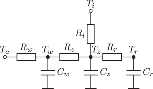
RC-model representing the thermal dynamics of one zone.
Reformulating (20) into (1) results in the state vector
3.1 Modeling solar radiation
Solar radiation has a major impact on the temperature inside buildings. Thus, considering the heat gain from radiation is a great opportunity to reduce the energy demand. Computing the aforementioned heat gain introduces several sources of uncertainty, starting at the radiation measurements. The required quantities are Direct Normal Irradiation (DNI), Diffuse Horizontal Irradiation (DHI) and Global Horizontal Irradiation (GHI). DNI is the radiation on a surface normal to the sun. It is measured with a solar tracker and a pyrheliometer which is labor-intensive. DHI is the diffuse, reflected radiation from the surrounding. Here, a pyranometer can be used with a shading device to block the direct sun beam. GHI is the global radiation and is measured with a pyranometer placed horizontally on a surface [23], [24]. These measured variables are related with
where z is the sun zenith angle [25]. Since GHI is significantly easier to obtain, the majority of on-site measurements are GHI and no information about DNI and DHI is available. Many correlations exist to obtain estimates for DNI and DHI from GHI. A comparison can be found in [25].
The tilted irradiation I
t
in
with the angle θ as the sun altitude, R d as the diffuse transposition factor of ground reflection, ρ for the foreground albedo and R r as the transposition factor for ground reflection. Under the isotropic assumption, the transposition factors R r and R d can be computed with
where s is the tilt angle of the surface. Note that for R d this is a rather strong assumption which is outlined in [25].
With the tilted irradiation I
t
, one can compute the heat gain
is used, where A win is the window surface area with the reflection factor R win. Note that the explicit time dependence of (24) and (26) was dropped for brevity.
4 Evaluation
In this section, we evaluate the application of LFMs and SMPC to Building Energy Systems, where solar radiation is considered as a disturbance.
4.1 Use cases
Two BES are taken into account: An example building in EnergyPlus and a parametric model of a floor at the Bosch Research Campus in Renningen, Germany. Ideal HVAC equipment was used for both use cases, since only the energy demand of the zones were of interest. The differences are outlined in the following.
4.1.1 EnergyPlus model
EnergyPlus is a widely adopted BES simulation software used by engineers to e.g. estimate and configure the HVAC equipment [13]. It provides a complex calculation of the thermal properties of a building, including the various disturbances and interactions with the HVAC components. EnergyPlus supplies typical weather data for different regions on earth, which are used during simulation. Thus, it is a white-box modelling approach for BES.
For the simulations in EnergyPlus, the building in Figure 3 is considered. It consists of three adjacent zones, the south, hallway and north zone, where the south and north zones are offices. For the control, every zone is modeled by (20) with identified values for the heat capacities and resistances from simulated data. As said before, EnergyPlus provides typical weather data for different climate zones. Here, typical data from Munich was used. Through the typical weather data, values for DNI, DHI and GHI are available for computing the heat gain through solar radiation.
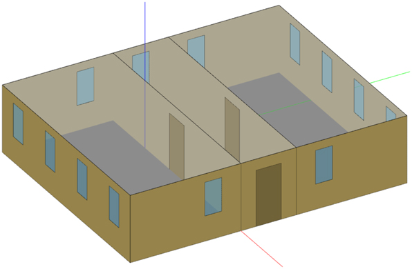
3D view of the example building in EnergyPlus.
4.1.2 Renningen office floor
The Renningen model is based on the floor plan shown in Figure 4. It also uses the model in (20) without explicit zone couplings and identified parameters from real world measurements. These measurements include weather data, where only the ambient temperature and GHI are available. From all available zones, only 9, 10, 21 and 23 are used, since 11, 12 and 13 are not subject to solar radiation. Zone 22 and 24 are not used since the thermal characteristics match zone 23 and 21, respectively. From this real world example information about the used RB controller is available, which is used for comparison in the evaluation. It consists out of two PI-Controllers, one for the radiator and one for the ventilation. The setpoint changes between night and day are smoothed with a ramp, so no abrupt changes occur, like in [4].
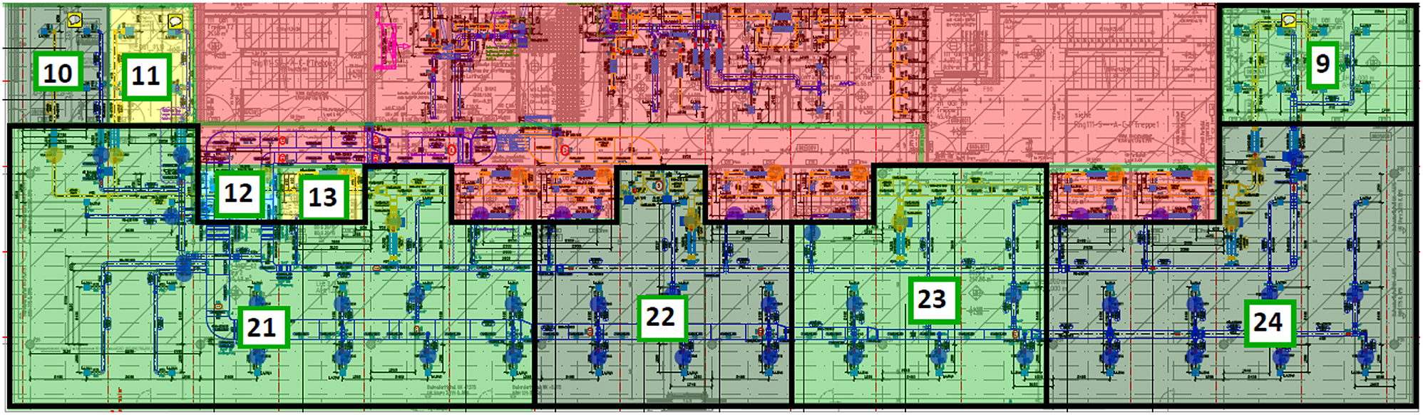
Zone layout of the floor at the Bosch research campus in Renningen.
4.2 Solar radiation prediction
From the building perspective, solar radiation, like ambient temperature, is a time dependent disturbance. As seen in Section 3.1, DNI, DHI and GHI are required for computing the heat gain
The computed heat gain for one zone in Renningen can be seen in Figure 5. Here, the signal properties of the disturbance are evident. A daily periodic trend with variations can be seen with a rough shape. Thus, a combination of a periodic and a Matérn kernel, a quasi-periodic kernel, is a suitable choice. For the Matérn kernel,
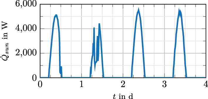
Computed heat gain through solar radiation with α = 1.
4.3 SMPC settings
The stochastic model predictive controller is implemented using the framework GRAMPC-S [28]. GRAMPC-S provides several approximation methods to propagate the uncertainties of the predicted states. In our evaluation, the unscented transformation with α UT = 0.1, β = 2 and κ = 1 is used to track the variance of the system dynamics. A diffusion term of 1E−5 K is added to both systems for the uncertainty propagation which resembles uncertain system dynamics. The parameters for the MPC models were identified from simulation data.
The temperature of each zone is subject to the constraints
where T
u
is the upper and T
l
the lower bound. The bounds are found in Table 1 which specify the comfort range during the day and energy efficiency for the night. Lower temperatures can result in condensation and thus yield mold, which is undesired. For the SMPC, Gaussian chance constraint approximations with the probabilities
for every control input u i to ensure energy efficiency.
Constraints for Comfort and Economy mode.
| Time | 6 am to 6 pm | 6 pm to 6 am |
|---|---|---|
| T u | 24 °C | 28 °C |
| T l | 21 °C | 17 °C |
The solar radiation is considered in two different ways: As a constant disturbance and with an LFM. An SMPC without disturbance knowledge is used as a baseline. Combined with the different probabilities of constraint fulfillment, 9 different controllers are considered and simulated for a whole year. They are compared based on the zones’ energy demand and thermal comfort levels. The discomfort is assessed with the integrated constraint violation given in K h. The different settings of the SMPC such as sample time and prediction horizon are shown in Table 2.
MPC settings for EnergyPlus and Renningen.
| EnergyPlus | Renningen | |
|---|---|---|
| dt | 5 min | 15 min |
| T hor | 2 h | 1 h |
|
|
10 | 1 |
|
|
50 | 10 |
4.4 Renningen results
The results for Renningen are given in Figure 6. Additionally, a time series plot is shown in Figure 7 which shows the SMPC with α = 95 % with a constant disturbance prediction. Overall for α = 95 % result in the highest energy consumption followed by α = 80 % and α = 50 %. When looking at the discomfort, α = 95 % achieve the lowest followed again by α = 80 % and α = 50 %. Including a constant disturbance prediction reduces both energy demand and discomfort, except for zone 21. Here a small increase in Energy consumption occurs. With the constant disturbance prediction, α = 50 % results in the lowest energy consumption for each zone. For α = 95 % in the zones 9 and 10, this effectively results in no discomfort. The effect for zone 21 and 23 is much smaller than expected. Further investigation shows, that the ventilation for these zones is at its upper control limit. This can also be seen in Figure 7. The influence of the solar radiation is greater, since the windows of zone 21 and 23 are facing south. Nevertheless, the discomfort is at least halved with the constant disturbance prediction.
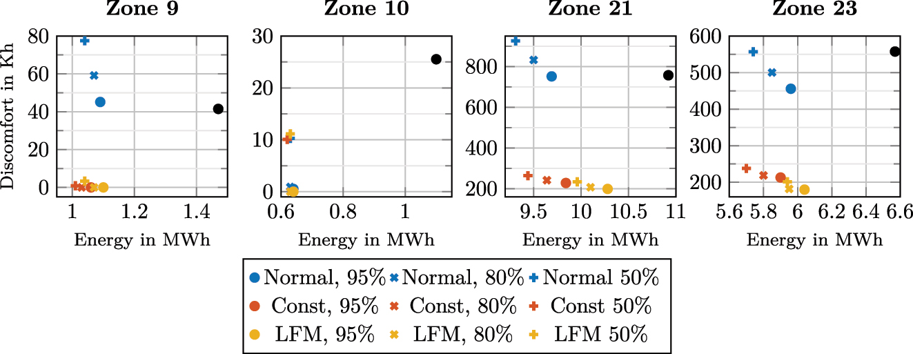
Renningen results for a prediction horizon of 1 h. The RB controller is depicted by  .
.
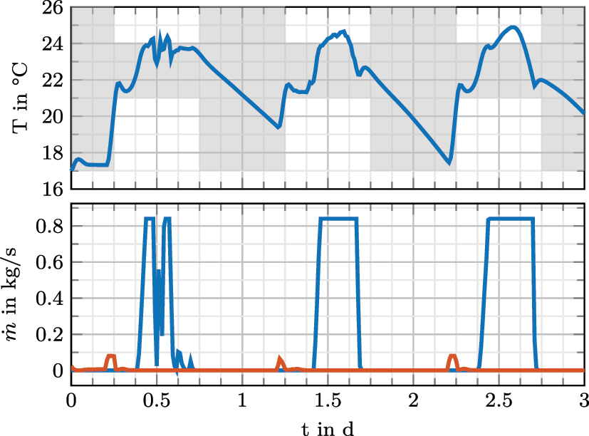
Time series result for zone 21 with α = 95 % and constant disturbance prediction. The lower plot shows the controls u
a
( ) and u
w
(
) and u
w
( ). The shaded area depicts the admissible temperature range.
Using an LFM to stochastically predict the solar heat gain results in a higher or comparable energy consumption for the zones. For zone 9 and 10 this results in a marginally higher energy consumption than the constant prediction. In zone 21 and 23, the discomfort for
Comparing with the RB controller, the SMPC at least reduces the energy demand for every zone. Including disturbance information leads to an additional reduction in discomfort.
Overall, the LFM results in a lower discomfort at the price of marginal higher energy consumption compared to the constant disturbance prediction. When a low discomfort is desired, the LFM is clearly the best choice. If energy efficiency is the biggest concern, a constant disturbance prediction with α = 50 % performs best. Note again that for α = 50 % and a Gaussian constraint approximation, the SMPC result is equivalent to a deterministic MPC, see Section 4.3.
4.5 EnergyPlus results
The EnergyPlus use case was simulated with a time horizon of 2 h with the results given in Figure 8. A similar trend like in the Renningen case can be seen. The constant disturbance prediction achieves a lower discomfort for α = 50 % compared to the LFM. In contrast, the energy consumption is slightly larger. Using an LFM results in a considerably lower discomfort for α = 95 % and α = 80 % with a higher energy consumption of about 4–8 %.
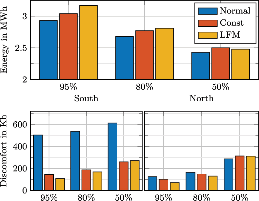
EnergyPlus results for a prediction horizon of 2 h.
To further assess the performance of the SMPC, the complementary cumulative constraint violation is shown in Figure 9. For the south, the SMPC without disturbance information has a significantly greater proportion of high constraint violations. Including a constant disturbance prediction reduces this probability significantly. This is different for the northern zone. Here, the SMPC is grouped in clusters of their chance constraint approximation percentage, e.g. for α = 95 % the performance between no disturbance prediction, constant prediction and LFM is similar. Thus, the advantage of adding disturbance information is smaller for the north zone than for the south zone.This meets the expectation that solar radiation has a lower impact on the northern zone. Moreover, model uncertainties are more dominant in the north, resulting in a higher discomfort for α = 50 %.
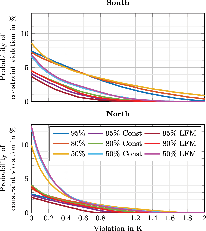
Complementary cumulative distribution of the constraint violation for 2 h.
5 Conclusions
This paper demonstrates the application of Latent Force Models (LFM) combined with SMPC to Building Energy Systems (BES). The LFM-based SMPC achieves the lowest discomfort in most cases. Additionally, the higher energy consumption appears reasonable for the comfort gained. When parameters are known exactly, a deterministic MPC still yields the lowest energy consumption.
Comparing deterministic and stochastic MPC, the main drawback of SMPC is its higher computational demand. To track uncertainty, at least the covariance of the states must be computed, resulting in at least quadratic computational scaling. This can become intractable, especially for BES with a large number of states. The primary advantage of SMPC over MPC is its stochastic treatment of constraints, leading to a natural tightening based on present uncertainties.
Future work includes refining the parameter identification process. Currently, only point estimates with a Wiener process are used, which does not accurately capture model uncertainties. Using a maximum a posteriori estimate would define a prior distribution for the parameters, considering their stochastic nature, which could further reduce discomfort. Another direction is the stochastic treatment of constraints. A heuristic method for constraint tightening could be developed to circumvent the additional computational demand of SMPC.
About the authors

Thore Wietzke is a research assistant at the Chair of Automatic Control at Friedrich-Alexander-Unversität Erlangen-Nürnberg. His research focuses on system identification with machine learning and nonlinear model predictive control for building energy systems.

Daniel Landgraf is a research assistant at the Chair of Automatic Control at Friedrich-Alexander-Unversität Erlangen-Nürnberg. His main focus is stochastic model predictive control with uncertainty aware machine learning.

Prof. Dr.-Ing. Knut Graichen is head of the Chair of Automatic Control at Friedrich-Alexander-Universitat Erlangen-Nurnberg. Main research areas: model predictive and distributed control as well as machine learning methods for control with applications in mechatronics, robotics, and energy systems. Knut Graichen is Editor-in-Chief of Control Engineering Practice.
-
Research ethics: Not applicable.
-
Informed consent: Not applicable.
-
Author contributions: All authors have accepted responsibility for the entire content of this manuscript and approved its submission.
-
Use of Large Language Models, AI and Machine Learning Tools: LLMs were used to improve the reading flow in the introduction. AI-assisted translations were used throughout the manuscript.
-
Conflict of interest: The authors state no conflict of interest.
-
Research funding: Funded by the German Federal Ministry for Economic Affairs and Climate Action under grant number 03EN1066B.
-
Data availability: Not applicable.
References
[1] IEA, “Buildings,” Tech. Rep., IEA, 2022. Available at: https://www.iea.org/reports/buildings.Suche in Google Scholar
[2] J. Clauß, C. Finck, P. Vogler-Finck, and P. Beagon, “Control strategies for building energy systems to unlock demand side flexibility – a review,” in Proceedings of Building Simulation 2017: 15th Conference of IBPSA, 2017.10.26868/25222708.2017.462Suche in Google Scholar
[3] W. O’Brien, I. Gaetani, S. Gilani, S. Carlucci, P.-J. Hoes, and J. Hensen, “International survey on current occupant modelling approaches in building performance simulation,” J. Build. Perform. Simul., vol. 10, nos. 5–6, pp. 653–671, 2017. https://doi.org/10.1080/19401493.2016.1243731.Suche in Google Scholar
[4] P. Stoffel, L. Maier, A. Kümpel, T. Schreiber, and D. Müller, “Evaluation of advanced control strategies for building energy systems,” Energy Build., vol. 280, nos. 0378-7788, p. 112709, 2023. https://doi.org/10.1016/j.enbuild.2022.112709.Suche in Google Scholar
[5] M. A. Álvarez, D. Luengo, and N. D. Lawrence, “Linear latent force models using Gaussian processes,” IEEE Trans. Pattern Anal. Mach. Intell., vol. 35, no. 11, pp. 2693–2705, 2013. https://doi.org/10.1109/tpami.2013.86.Suche in Google Scholar PubMed
[6] C. E. Rasmussen and C. K. I. Williams, Gaussian Processes for Machine Learning, Cambridge, Massachusetts, MIT Press, 2005.10.7551/mitpress/3206.001.0001Suche in Google Scholar
[7] J. Hartikainen and S. Särkkä, “Kalman filtering and smoothing solutions to temporal Gaussian process regression models,” in 2010 IEEE International Workshop on Machine Learning for Signal Processing, 2010, pp. 379–384.10.1109/MLSP.2010.5589113Suche in Google Scholar
[8] S. Särkkä, M. A. Álvarez, and N. D. Lawrence, “Gaussian process latent force models for learning and stochastic control of physical systems,” IEEE Trans. Autom. Control, vol. 64, no. 7, pp. 2953–2960, 2019. https://doi.org/10.1109/tac.2018.2874749.Suche in Google Scholar
[9] J. Graßhoff, G. Männel, H. S. Abbas, and P. Rostalski, “Model predictive control using efficient Gaussian processes for unknown disturbance inputs,” in Proc. 2019 IEEE 58th Conference on Decision and Control (CDC), 2019, pp. 2708–2713.10.1109/CDC40024.2019.9030032Suche in Google Scholar
[10] D. Landgraf, A. Völz, and K. Graichen, “Nonlinear model predictive control with latent force models,” in Proc. 2022 American Control Conference (ACC), 2022, pp. 4979–4984.10.23919/ACC53348.2022.9867650Suche in Google Scholar
[11] T. Wietzke, J. Gall, and K. Graichen, “Occupancy prediction for building energy systems with latent force models,” Energy Build., vol. 307, nos. 0378-7788, p. 113968, 2024. https://doi.org/10.1016/j.enbuild.2024.113968.Suche in Google Scholar
[12] F. Oldewurtel, et al.., “Energy efficient building climate control using stochastic model predictive control and weather predictions,” in Proc. 2010 American Control Conference, 2010, pp. 5100–5105.10.1109/ACC.2010.5530680Suche in Google Scholar
[13] EnergyPlus, “Energyplus v22.1.0 engineering reference,” Tech. Rep., U.S. Department of Energy, 2022.Suche in Google Scholar
[14] E. Klenske, M. N. Zeilinger, B. Schölkopf, and P. Hennig, “Gaussian process-based predictive control for periodic error correction,” IEEE Trans. Control Syst. Technol., vol. 24, no. 1, pp. 110–121, 2016. https://doi.org/10.1109/tcst.2015.2420629.Suche in Google Scholar
[15] A. Solin and S. Särkkä, “Explicit link between periodic covariance functions and state space models,” in Proc. Seventeenth International Conference on Artificial Intelligence and Statistics, S. Kaski and J. Corander, Eds., vol. 33 of Proceedings of Machine Learning Research, (Reykjavik, Iceland), PMLR, 2014, pp. 904–912.Suche in Google Scholar
[16] S. Särkkä, “On unscented Kalman filtering for state estimation of continuous-time nonlinear systems,” IEEE Trans. Autom. Control, vol. 52, no. 9, pp. 1631–1641, 2007. https://doi.org/10.1109/tac.2007.904453.Suche in Google Scholar
[17] C. Gardiner, Stochastic Methods, vol. 4, Berlin Heidelberg, New York, Springer, 2009.Suche in Google Scholar
[18] D. Landgraf, A. Völz, F. Berkel, K. Schmidt, T. Specker, and K. Graichen, “Probabilistic prediction methods for nonlinear systems with application to stochastic model predictive control,” Ann. Rev. Control, vol. 56, 2023, Art. no. 1367-5788, https://doi.org/10.1016/j.arcontrol.2023.100905.Suche in Google Scholar
[19] G. C. Calafiore and L. E. Ghaoui, “On distributionally robust chance-constrained linear programs,” J. Optim. Theor. Appl., vol. 130, nos. 1573–2878, pp. 1–22, 2006. https://doi.org/10.1007/s10957-006-9084-x.Suche in Google Scholar
[20] K. B. Jemaa, P. Kotman, and K. Graichen, “Model-based potential analysis of demand-controlled ventilation in buildings,” IFAC-PapersOnLine, vol. 51, no. 2, pp. 85–90, 2018. https://doi.org/10.1016/j.ifacol.2018.03.015.Suche in Google Scholar
[21] F. Massa Gray and M. Schmidt, “Thermal building modelling using Gaussian processes,” Energy Build., vol. 119, nos. 0378-7788, pp. 119–128, 2016. https://doi.org/10.1016/j.enbuild.2016.02.004.Suche in Google Scholar
[22] K. Arendt, M. Jradi, H. Shaker, and C. Veje, “Comparative analysis of white-, gray- and black-box models for thermal simulation of indoor environment: teaching building case study,” in Proc. 2018 Building Performance Analysis Conference and SimBuild Co-Organized by ASHRAE and IBPSA-USA, vol. 8 of SimBuild Conference, Chicago, USA, ASHRAE/IBPSA-USA, 2018, pp. 173–180.Suche in Google Scholar
[23] J. L. Balenzategui, F. Fabero, and J. P. Silva, Solar Radiation Measurement and Solar Radiometers, Berlin Heidelberg, New York, Springer International Publishing, 2019, pp. 15–69.10.1007/978-3-319-97484-2_2Suche in Google Scholar
[24] C. A. Gueymard and D. R. Myers, Solar Radiation Measurement: Progress in Radiometry for Improved Modeling, Berlin, Heidelberg, Springer Berlin Heidelberg, 2008, pp. 1–27.10.1007/978-3-540-77455-6_1Suche in Google Scholar
[25] C. A. Gueymard, “Direct and indirect uncertainties in the prediction of tilted irradiance for solar engineering applications,” Sol. Energy, vol. 83, no. 3, pp. 432–444, 2009. https://doi.org/10.1016/j.solener.2008.11.004.Suche in Google Scholar
[26] Y. Zhang, E. Long, Y. Li, and P. Li, “Solar radiation reflective coating material on building envelopes: heat transfer analysis and cooling energy saving,” Energy Explor. Exploit., vol. 35, no. 6, pp. 748–766, 2017. https://doi.org/10.1177/0144598717716285.Suche in Google Scholar
[27] J. Orgill and K. Hollands, “Correlation equation for hourly diffuse radiation on a horizontal surface,” Sol. Energy, vol. 19, no. 4, pp. 357–359, 1977. https://doi.org/10.1016/0038-092x(77)90006-8.Suche in Google Scholar
[28] D. Landgraf, A. Völz, and K. Graichen, “A software framework for stochastic model predictive control of nonlinear continuous-time systems (GRAMPC-S),” 2024 [Online]. Available at: https://arxiv.org/abs/2407.09261.Suche in Google Scholar
© 2025 the author(s), published by De Gruyter, Berlin/Boston
This work is licensed under the Creative Commons Attribution 4.0 International License.
Artikel in diesem Heft
- Frontmatter
- Editorial
- Data-driven and learning-based control – perspectives and prospects
- Methods
- Towards explainable data-driven predictive control with regularizations
- Two-component controller design to safeguard data-driven predictive control
- Robustness of online identification-based policy iteration to noisy data
- Koopman-based control of nonlinear systems with closed-loop guarantees
- Applications
- Data-driven feedback optimization for particle accelerator application
- Application of stochastic model predictive control for building energy systems using latent force models
- Learning-based model identification for greenhouse climate control