Learning-based model identification for greenhouse climate control
-
Michael Fink
 ,
Annalena Daniels
,
Annalena Daniels

Abstract
A controller for the air temperature and relative humidity of a greenhouse is presented that relies only on the efficient exploitation of natural ventilation. Due to the difficulty of modeling greenhouse climate from first principles, Neural Predictive Control (NPC) is chosen, which combines the advantages of learning with Model Predictive Control (MPC) under constraints. Feedforward Neural Networks (NNs) are used to obtain a predictive model and a simulation model for the complex nonlinear dynamics of the temperature and humidity inside a greenhouse. The NNs are trained and validated with an 81-day dataset recorded in a Mediterranean greenhouse. The MPC approach applies operational constraints to compute the optimal vent opening. It minimizes temperature and humidity tracking errors, limits control increments to reduce motor wear, and enforces soft bounds on greenhouse temperature and humidity. Hard constraints include vent saturation and a wind speed limit for safety. The NPC strategy was evaluated in simulation with real weather, featuring both sunny and windy conditions. The results show small validation errors of the NNs. The tracking error in the control approach in situations without saturated input is below 3 K and in 81 % of the time the humidity is within the bounds. The presented data-driven control approach is attractive for controller design as data availability in greenhouses is expected to increase in the coming years.
Abstract
Ein Regler für die Lufttemperatur und relative Luftfeuchtigkeit in einem Gewächshaus wird vorgestellt, der ausschließlich auf die effiziente Nutzung der natürlichen Belüftung setzt. Aufgrund der Schwierigkeit, das Gewächshausklima aus physikalischen Grundlagen heraus zu modellieren, wird Neural Predictive Control (NPC) eingesetzt, eine Methode, die die Vorteile des maschinellen Lernens mit denen der modellprädiktiven Regelung (MPC) unter Einhaltung von Nebenbedingungen kombiniert. Vorwärtsgerichtete Neuronale Netze (NNs) werden verwendet, um sowohl ein Vorhersagemodell als auch ein Simulationsmodell für die komplexen, nichtlinearen Dynamiken von Temperatur und Luftfeuchtigkeit im Inneren des Gewächshauses zu erstellen. Die neuronalen Netze werden mit einem über 81 Tage aufgezeichneten Datensatz aus einem mediterranen Gewächshaus trainiert und validiert. Der MPC-Ansatz berücksichtigt betriebliche Einschränkungen, um die optimale Fensteröffnung zu berechnen. Dabei werden Temperatur- und Feuchtigkeitsabweichungen minimiert, Steuerungsänderungen begrenzt, um den Verschleiß der Antriebe zu reduzieren, und weiche Schranken für Temperatur und Luftfeuchtigkeit im Gewächshaus eingehalten. Harte Nebenbedingungen umfassen die Begrenzung der Fensteröffnung sowie eine Windgeschwindigkeitsgrenze aus Sicherheitsgründen. Die NPC-Strategie wurde in einer Simulation mit realen Wetterdaten getestet, die sowohl sonnige als auch windige Bedingungen umfasste. Die Ergebnisse zeigen geringe Validierungsfehler der neuronalen Netze. Der Regelabweichungsfehler liegt in Situationen ohne gesättigte Eingaben unter 3 K, und in 81 % der Zeit bleibt die Luftfeuchtigkeit innerhalb der vorgegebenen Grenzen. Der vorgestellte datengetriebene Regelungsansatz ist vielversprechend für die Reglerauslegung, da in den kommenden Jahren mit einer steigenden Datenverfügbarkeit in Gewächshäusern zu rechnen ist.
1 Introduction
In modern agriculture, precise control of environmental conditions is essential to optimize the productivity of greenhouse crops. A greenhouse is a structure designed to create a controllable environment that favors the growth of crops, protecting them from adverse climatic factors and pests. Thanks to their transparent materials, such as glass or plastic, greenhouses allow sunlight to enter, which is crucial for crop photosynthesis. Climate control systems, such as ventilation and heating, can be installed in a greenhouse to maintain a stable environment for plants, keeping conditions within a specific range regardless of outside weather changes. The use of automatic control techniques is crucial for regulating variables such as temperature and humidity to ensure the healthy growth of plants and fruit. In particular, automatic control allows for quick adjustments to external weather changes, ensuring a consistently stable microclimate within the greenhouse [1].
In Mediterranean greenhouses, natural ventilation is the main action for farmers to control the temperature and humidity due to the mild climate of the region and the low cost of this approach. Natural ventilation is the exchange of air between the inside and outside of a greenhouse without other technical assistance, such as fans or air conditioning. The temperature needs to be controlled to avoid too high or too low temperatures, negatively affecting fruit development. The relative humidity must stay within reasonable bounds to prevent plant water stress and the appearance of fungal disease [2]. Thus, the opening of the greenhouse vents must be controlled when the inside conditions get unfavorable so that warm air can escape while cooler air enters, promoting an airflow that also allows for the exchange of humid air [3]. Designing an effective controller benefits greatly from an accurate model, yet the greenhouse environment is influenced by highly nonlinear and tightly coupled factors [4] such as external weather conditions (e.g., temperature and air pressure affect humidity) and internal variables such as greenhouse structure, size, and crop types. This complexity makes identification from first principles challenging, and even a well-defined model often applies only to a specific greenhouse under specific weather conditions. When conditions change, model and controller parameters must be recalibrated. These complexities make greenhouse climate control a challenging control engineering problem.
Various control techniques have been proposed for greenhouse control [1], [5], [6]. These include PID control with and without feedforward component [7], [8], [9], adaptive control [10], [11], [12], selective and event-based control [13], fuzzy control [14], and nonlinear control [15], [16] including Model Predictive Control (MPC) approaches [17], [18], [19]. A common approach is to track only a reference temperature while maintaining humidity within acceptable ranges for the crop. When humidity exceeds these ranges, the temperature setpoint is changed to force the vents to open which enables the exchange of humid air [1]. Although the above techniques have proven to be effective, they have some drawbacks. On the one hand, PID control (and other approaches based on PID control) rely on low-order models identified for the dynamics of the greenhouse microclimate, which changes over the year and for every greenhouse and region, thus requiring repeated tuning of the controller parameters and/or repeated model identification. On the other hand, adaptive and nonlinear control techniques require knowledge of the dynamics that relate temperature and humidity to the natural ventilation effect, for example, in the form of first-principles-based models. While these models can capture the environment dynamics, in reality, they still need repeated recalibrations [20]. In this sense, the expressions relating the greenhouse microclimate and the ventilation effect are strongly nonlinear [4], which makes them complex to use to develop control strategies analytically.
Among the control methods discussed, MPC is one of the most promising ones for greenhouse climate control because it combines the ability to handle complex, multivariable dynamics with constraint satisfaction properties. By predicting future conditions, MPC optimizes control actions over a given horizon, effectively managing temperature and humidity while integrating operational constraints to ensure safe, efficient control that minimizes equipment wear. However, a major drawback of MPC is that it requires an accurate model to perform optimally, and as mentioned developing such a model is challenging due to the complex and changing nature of greenhouse environments.
In recent years, learning-based control techniques have been applied to handle complex dynamics like these, opening up the possibility of using MPC efficiently for greenhouses. An overview of learning-based MPC methods is provided in [21], and a demonstration of a state-of-the-art Neural Network (NN)-based MPC, also known as Neural Predictive Control (NPC), applied to robotics, is presented in [22]. These data-driven modeling and control techniques have also been applied to manage the complex dynamics of the greenhouse microclimate, e.g., by approaches using linear MPC [23], [24]. The application of NPC for greenhouses is explored in [25], where heating is used alongside vents as an input, facilitating easier control but at increased operational cost. In contrast [26], uses only vent control to manage temperature, though this approach does not account for indoor humidity, which significantly simplifies the learning and control part. For learning of an NN, the approach in [27] relies on artificially generated data based on an analytical model, which may not fully capture the variability of real-world greenhouse conditions.
However, datasets with a relevant amount of measurements are required for the development of learning-based control, which has previously been a limitation. An increasing number of greenhouses are being equipped with data acquisition systems that are connected to cloud computing platforms [28], [29]. Therefore, it is expected that data availability will not be the limiting factor anymore in the coming years [30]. This work aims to take advantage of these future developments by using greenhouse data to implement a temperature and humidity control technique based directly on measured data, eliminating the need for explicit mathematical models. This approach simplifies the modeling of complex dynamics and ensures that the method is applicable across different greenhouses without the need for extensive model identification, while retaining the benefits of MPC.
1.1 Problem statement and contribution
The objective of this work is to maintain optimal temperature and humidity in a greenhouse using natural ventilation. This task is challenging due to the complex, nonlinear interactions between indoor climate variables and external weather conditions, which vary by region and depend on greenhouse-specific factors such as orientation with respect to the wind and sun and structure of the greenhouse. In addition, simultaneous control of temperature and humidity often results in conflicting control actions, requiring weighted cost functions. Safety mechanisms are essential to prevent unsafe conditions, such as open vents during strong winds.
In contrast to existing data-driven approaches that use simplified linear models [23], [24] or artificially generated data [27], this work proposes a fully data-driven nonlinear MPC that learns directly from real greenhouse data. Compared to prior neural-network-based MPC methods [26], which focus solely on temperature, this approach jointly optimizes temperature and humidity while accounting for their coupled dynamics and constraints.
The main contribution of this work is the integration of all these factors into a single method, addressing gaps left by previous approaches and advancing state-of-the-art greenhouse climate control. This is achieved through a learning-based MPC strategy to regulate greenhouse temperature and humidity using natural ventilation. In this context, the term “learning-based” refers to approaches in which the system dynamics is represented by machine learning models, such as NNs. Unlike traditional models, which require frequent recalibration, and prior data-driven models that rely on pre-generated datasets, the approach presented in this work enables continuous adaptation to the changing greenhouse conditions, such as changes in dynamics due to seasonal changes or wear. NNs were chosen over other learning-based approaches for this application due to the need for scalability, transfer learning, and online learning capabilities in greenhouse environments to allow for automatic adjustments to the current region and structure [31], [32]. The NPC strategy is tested in simulation using weather data from a traditional greenhouse in Southeastern Spain.
1.2 Paper outline
The remainder of this paper is structured as follows: Section 2 describes the greenhouse setup and the experimental data used for model learning. The background of learning-based MPC is explained, including NN modeling approaches. The proposed NPC strategy for greenhouse climate control is then presented in Section 3, covering the identification of the environmental model and the design of the control framework. Section 4 presents and discusses the results. Finally, Section 5 summarizes the main findings.
1.3 Notation
Vectors are written as bold lowercase letters, matrices are denoted as bold uppercase letters, and sets are denoted with calligraphic font, e.g.,
x
,
A
, and
2 Materials and methods
2.1 Greenhouse data
The data used in this work is from the greenhouse shown in Figure 1, located at “Las Palmerillas” Experimental Station of the Cajamar Foundation, in El Ejido, Almería, Spain. It is a traditional Almería-type greenhouse with an area of 877 m2 (37.80 m × 32.20 m) and a polyethylene cover. The greenhouse is equipped with several actuation systems that control the climate. In particular, the natural ventilation system consists of five roof vents (8.36 m × 0.73 m) and two lateral vents (32.75 m × 1.90 m) on the north and south sidewalls. As shown in Figure 1, the roof vents have an angled opening and the lateral vents are opened by rolling up a plastic film. The vents are motor-controlled and can be opened from 0 % to 100 % of their ventilation area.

Traditional Almería-type greenhouse.
The main climatic variables were recorded every 30 s using two sensors (each measuring both temperature and humidity). One is placed outside and one inside central in the greenhouse. The following variables were measured for this work: solar global radiation R in
The opening ratio of each vent in %, u ven, was recorded every 30 s, as the electric motors are connected to a supervisory and control data acquisition (SCADA) system in which manual and automatic actions are performed to regulate the air temperature inside the greenhouse by natural ventilation.
Formally, for a given time k, the input u
k
= u
ven,k
is the opening percentage, meaning that at 100 % all windows are fully open and at 0 % they are fully closed. All windows are controlled identically, so u
ven,k
is a scalar value applied to each window. For a traditional low-tech greenhouse, there are no other actuators that heat, cool, humidify, or dehumidify the greenhouse. The state of the greenhouse is described by
The next section introduces NPC which is a standard learning-based MPC.
2.2 Learning-based model predictive control
For prediction of the state sequence for a specified input sequence, the system dynamics are modeled using a nonlinear discrete-time state-space representation
where
2.2.1 Model predictive control
MPC is a control method that optimizes future inputs of a system by predicting the state trajectory over a time horizon
2.2.2 Modeling with neural networks
In contrast to physics-based models that rely on the analytical description of systems dynamics, NNs indirectly capture these mappings and correlations based on the data they see, making them an attractive option for the modeling of systems and for model-based control methods.
In this work, a simple feedforward NN is used to model the system dynamics update, with a mapping from input data
The input data
d
k
is weighted by
The parameterization of a NN combines all weights in W and biases in b resulting in the parametrized function f ( d k , W , b ). In this setup, q represents the dimension of the input vector d k (i.e., the number of features), r is the number of neurons in each hidden layer, and s is the dimensionality of the output (i.e., the number of output neurons in h L ).
The next section describes how the NPC is adapted specifically for the given greenhouse data in order to fulfill the requirements given in Section 2.1.
3 Neural predictive control for greenhouses
In order to control the greenhouse climate with an NPC approach, two major design steps must be considered. First, the model for the controller must be learned, and thus, the data must be prepared to be used in a NN. As a second step, the NPC algorithm must be tuned according to the needs. This interplay is illustrated in the blue box in Figure 2. The optimal control problem of the NPC algorithm is based on a predictive NN that takes the current inside temperature and humidity x k , the weather data p k , and allowed vent opening percentages u k as inputs and predicts the corresponding changes in the state for the next time step Δ x k . The optimization finds a full sequence of future optimal vent configurations that result in good tracking performance for temperature and humidity regarding a specified reference x ref while never violating constraints. The predictive NN is chosen to have a large enough network to reproduce the main characteristics and dynamics of the greenhouse, but small enough to be computationally efficient, i.e., the parameterization of the predictive NN, given as f p, presents a trade-off between accuracy and function evaluation time. The model uses a coarser sampling time for the prediction, T p, than both the sampling rate of the motor controller for vent adjustments and the frequency of measurements taken in the greenhouse. This slower sampling rate is suitable because the dynamics of the greenhouse climate change slowly over time, allowing the model to make long-term predictions with reduced calculation time. Faster dynamics such as wind are handled by a safety layer in the controller in case a problem occurs between sampling times. The generated optimal inputs are applied to a more detailed simulation network, f s, which simulates the real greenhouse dynamics. This simulation network operates at the measurement sampling time of the greenhouse, T s. Since the simulation network is larger than the predictive network, there is a potential risk of overfitting. In order to mitigate this, k-fold cross validation and regularization techniques were employed, which will be explained in more detail in Section 3.1. Although both networks are trained on the same dataset, they are fundamentally different, to allow to mimic a scenario where the learning-based controller is applied for the real greenhouse. The prediction network is tailored to longtime prediction, the simulation network captures shorttime dynamics as well. The structure with two NN ensures that, on the one hand, the NPC is computationally feasible during optimization and, on the other hand, evaluated under realistic conditions. Details on the training of the two networks will be given in Section 3.1, and details on the NPC and on the optimization will be given in Section 3.2.
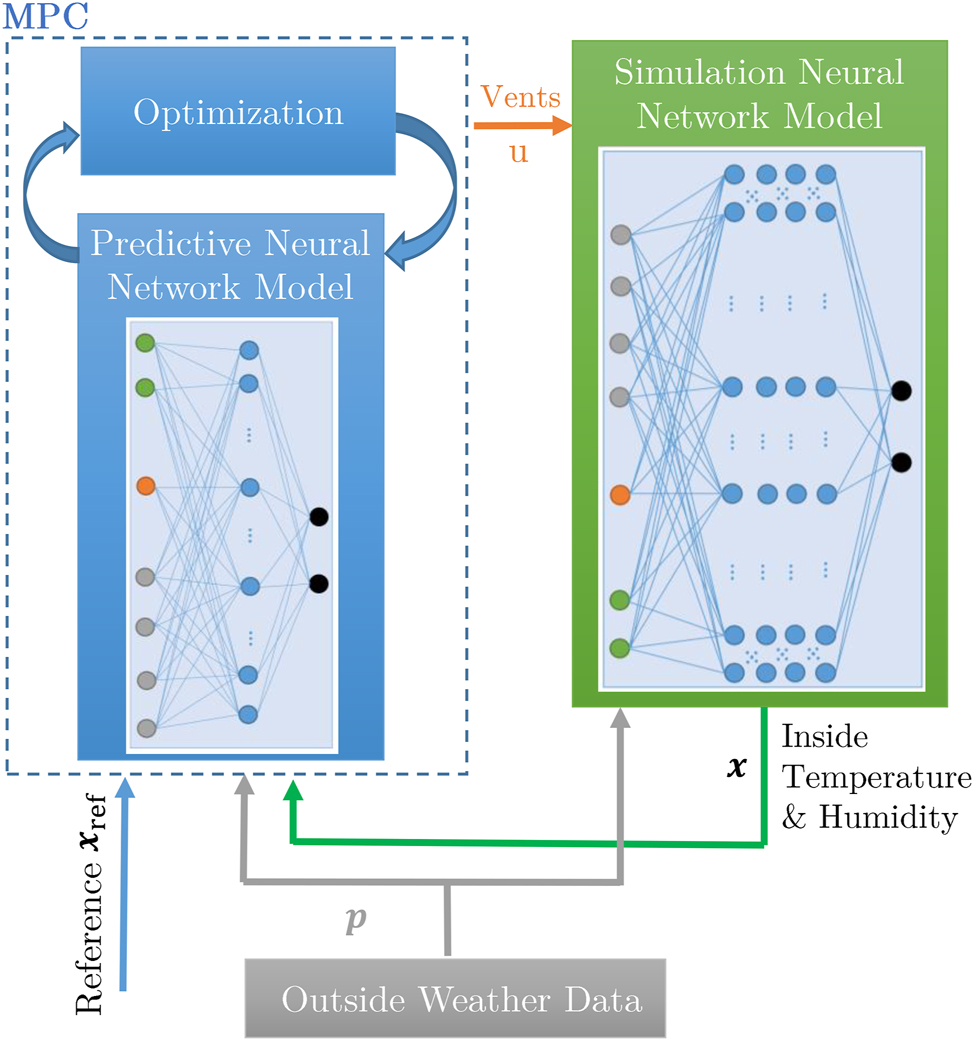
Overview of the NPC strategy. The controller generates inputs tested in the simulation model. At each time step, the optimization provides control inputs to bring states close to the reference values.
3.1 Greenhouse model identification
For the training of the NN model, it is essential to use a dataset containing the most informative data and with sufficient excitation for the relevant features. Note that in a greenhouse, the indoor climate is a consequence not only of the effect of the ventilation, but also of the external climate that acts as a disturbance. The excitation required to capture the dynamics of the indoor variables is therefore mainly imposed by the inherent variations of the external climate. As for the natural ventilation system, it has a strongly nonlinear effect on the indoor climate. Therefore, as shown in Figure 3, data with opening and closing of the greenhouse vents have been used, covering the whole actuator operation range. The vents remain open or closed for different intervals of time each day, and under different external climate conditions, especially wind speed, which significantly affects the ventilation effect.

Dataset for neural networks. Green background: data used for learning and validation in a k-fold cross-validation scheme; blue background: data solely used for testing.
Following an exploratory data analysis, relevant features were selected from the Mediterranean greenhouse data (see Section 2.1) to ensure that the model is trained on the most meaningful information, also ensuring coverage of diverse weather conditions. To that end, the dataset presented in Figure 3, comprising 81 days between October and December, was divided into three subsets: training data, validation data, and test data. The majority of the data (73 days, representing 90 % of the total data) was allocated for training and validation, while eight days from different weather scenarios were designated for testing. For training and hyperparameter tuning, a k-fold cross validation approach [34] was used with k = 5, meaning that in each ensemble, approximately 15 days out of the 73 were used for validation. Since this approach dynamically assigns training and validation data, it is not explicitly represented in Figure 3.
The following considerations were taken into account when using the data to synthesize the NN models. Although the greenhouse has roof and lateral vents, a single input is used to indicate the opening percentage of all the vents (i.e., all the vents are opened and closed at the same time). Similarly, internal radiation data is omitted as it follows external radiation, differing only by a factor influenced by the transmission coefficient of the cover. The inputs and outputs are then restructured to match the state-space representation, as shown in Figure 4. The network receives the data for one time step

Setup for neural network training. The network inputs are states, inputs, and parameters from the training. Its output predicts state changes for the next time step.
In contrast to the standard NN approaches, the proposed models of the greenhouse climate are in the form of a state space representation, and only the update of the state is modeled by the NN, as introduced in (1). The training was conducted in an open-loop setup, where the NN was trained using data from the dataset at each time step. The input of the NN is data from a single timestep, and the output is the state of the next time step, e.g., inside temperature and humidity. The chosen NNs for the predictive and simulation models are both feedforward networks composed of fully connected layers. The choice of activation functions
α
j
for each layer j should reflect the expected nonlinear dynamics. The predictive network is used in the gradient-based optimization of the MPC approach and must therefore remain differentiable, making the commonly used ReLU activation α(z) = max(0, z) unsuitable. Instead, the smooth approximation softplus activation
The presented identification method is applicable to all kinds of greenhouses if sufficient data is available, as it purely relies on the given data for a specific greenhouse.
3.2 Greenhouse climate control
Relying solely on the opening and closing of windows to track the desired indoor temperature and humidity reference simultaneously is a challenging task. This difficulty arises in particular because the single decision variable, the ratio at which the vents are open, has a significant impact on the humidity and the temperature, and the required control action for successful tracking of temperature and humidity is often in conflict. In order to obtain the best possible results for this trade-off in greenhouse climate control, optimal control is used, i.e., MPC, in combination with the NN models, as described in (1). Therefore, the proposed NPC problem is a specific adaptation of the general MPC framework, as described in Section 2.2.1, tailored to the specific needs of greenhouse climate control and is defined as follows
The optimization is based on the current measurement of the state
x
k
defined in (3e). Based on this measurement, the state trajectory is predicted with the learned predictive model (1), and the input trajectory results from minimizing the cost function J. The cost function J in (6) will be explained in Section 3.2.2. It contains a smoothing part, therefore it also requires the previous input, defined in the problem in (3f). The weather data
3.2.1 Constraints
When managing temperature and humidity in the greenhouse, operational restrictions must be included as constraints in the optimization process to ensure safe and realistic control inputs. In the optimization problem presented in (3), these constraints are introduced as hard constraints for inputs and states.
Vent openings are constrained to a feasible range of 0 %–100 %. Therefore, in the optimization the input is bounded by a hard constraint
In order to protect the greenhouse from structural damages, the vent position must be zero, i.e., closed vents, if the wind exceeds an upper bound, modeled by the hard constraint
The function
Due to the poor insulation of a greenhouse, the indoor climate often closely follows the external weather conditions, making it difficult to keep the greenhouse temperature and humidity hard-constrained. There is no guarantee that the external conditions will not enter phases that are highly unfavorable for plant growth. Enforcing hard constraints on system states is therefore impractical, since constraint satisfaction cannot be guaranteed. To ensure that the constraints are mostly satisfied, state constraints are included in the optimization problem only as soft constraints that penalize too large and too small temperature and humidity. Thus, the term
is included in the cost function with appropriate weights (detailed in the following Section 3.2.2), where
3.2.2 Cost function
The control goal for the greenhouse climate is defined by the cost function (6) over the prediction horizon N. It includes reference tracking, soft constraints, and a term that smoothens the control signal over time.
The cost function penalizes larger deviation from the reference temperature and reference humidity
x
ref, which are given as kth element of the reference trajectory
3.2.3 Adaption to day and night
Greenhouse conditions are strongly influenced by external weather, which fluctuates significantly, particularly between day and night. A significant contributing factor is the fact that greenhouses typically have only minor insulation, which allows sunlight to heat them during the day. This thin insulation, however, results in rapid cooling when outside temperatures drop, making it difficult to sustain daytime temperature levels overnight. The reference trajectory is designed based on the knowledge of the farmers. Since photosynthesis ceases without sunlight, and most plants do not require high temperatures at night, it is more efficient to lower the reference temperature during the night.
In order to achieve this, instead of a constant reference a sinusoidal temperature reference is used, setting a higher target during the day and a lower one at night. This approach minimizes large setpoint deviations at night and enhances controller performance, aligning it with plant requirements. For humidity, a constant tracking point is set at 70 % because the crop loses water if the humidity is too low and is at risk of disease if it is too high, regardless of day or night. However, the control priorities are adjusted by weighting temperature regulation more heavily during the day, when it is crucial, and focusing more on humidity control at night.
4 Results and discussion
The proposed method is evaluated using a simulation with weather data. Instead of deploying the controller in a physical greenhouse, it is tested on a simulation where the greenhouse dynamics are represented by f s. For offline training, the neural networks were run on a high-performance computer with 8 Tesla P100-PCIE-16GB GPUs and 2 AMD EPYC 7542 32-Core CPUs. The online control algorithm, including the optimization process, was run on a standard laptop with an 8-core AMD Ryzen 5 PRO 3500U processor.
First, in Section 4.1, the outputs of the greenhouse climate model are presented to demonstrate its accuracy and suitability for control purposes. Following in Section 4.2, the performance of the proposed controller is discussed when applied to the simulated greenhouse environment.
4.1 Data and modeling results
The predictive model f p is a fully connected NN with L p = 2 layers with r p = 64 neurons and a sampling time T p = 10 min. The p in the subscript, indicates the hyperparameter of the predictive model. The deeper and more accurate simulation network f s consists of L s = 4 layers with r s = 208 neurons each and the real-time sampling time of T s = 30 s, where the s in the subscript denotes parameter of the simulation model. This finer sampling interval is chosen as it aligns with the original 30 s sampling of the data, providing a more precise system model than that of the predictive network needed for the controller. In order to prevent overfitting, several regularization techniques were applied, including k-fold cross-validation (k = 5), dropout [37], learning rate reduction on plateaus, and weight decay. Training and validation losses were continuously monitored to detect early signs of overfitting, but no such issues were observed in the selected models. Further increasing the network size did not yield significant performance improvements. Both networks were trained using the mean squared error (MSE) loss with the Adam [38] optimizer. All hyperparameters, including the number of layers, neurons per layer, learning rate, weight decay, and dropout rate, were optimized using Optuna [39], which efficiently identified the best-performing configurations. This automated approach provides a more systematic and scalable optimization process compared to manual tuning. The selected hyperparameters include a weight decay of 6.71 × 10⁻⁶ for the predictive network and 1.95 × 10⁻⁶ for the simulation network, along with dropout rates of 0.1 and 0.125, respectively. The learning rates were set to 2.2 × 10⁻⁴ for the predictive network and 1.4 × 10⁻³ for the simulation network. The predictive network was trained for 850 epochs, while the simulation network underwent 750 epochs of training.
The networks were trained on the dataset presented in Figure 3, as explained in Section 3.1. The metrics for the test of both NNs are given in Table 1, which summarizes the mean, maximum, and variance of the absolute prediction errors for temperature and humidity. These metrics are computed solely for a one-step prediction, as the networks were trained to predict the state in the next time-step based on the current state and the current input. Both networks demonstrate strong performance, with the prediction network achieving low mean absolute errors of 0.080 K and 4.002 %pt for temperature and humidity, respectively, where %pt denotes percentage points. The simulation network also performs well, with minimal errors in both temperature (0.048 K) and humidity (4.442 %pt), indicating effective generalization to the test data.
Evaluation metrics for the neural networks on test data for a one-step prediction.
| NN | Prediction | Simulation | ||
|---|---|---|---|---|
| Temp. in K | Hum. in %pt | Temp. in K | Hum. in %pt | |
| Mean absolute error | 0.080 | 4.002 | 0.048 | 4.442 |
| Standard deviation | 0.100 | 4.895 | 0.067 | 5.838 |
| Maximum error | 0.238 | 14.988 | 0.198 | 16.255 |
| Variance of error | 0.010 | 21.570 | 0.003 | 33.924 |
Figure 5 presents results for test data. In the temperature and humidity plots, the gray line represents measured data, while the black and orange lines correspond to predictions from the NNs. Given the correct data from prior time steps, both networks closely match the actual dynamics for the next step. These results confirm that the model has effectively learned the training data, ensuring a highly accurate one-step prediction, which is an essential foundation for reliable multi-step forecasts and control applications. Since, in practice, predictions cannot rely on real measurements of the states for future time steps, the performance of the network is also evaluated over longer horizons without measurement updates. This is especially relevant for the prediction network that will be used in the NPC controller. However, in this work, the control method will be tested in a closed-loop simulation with the simulation network, making the accuracy of the simulation network relevant as well.

Model evaluation on test data. The test includes the performance of the model on days 3–6, with corresponding weather conditions and the vent inputs used during this period.
Figure 6 shows this evaluation for both networks. Both networks effectively capture the dynamics over the extended prediction horizon, although they both show slight deviations from the real data. On average, the simulation network remains closer to the actual temperature values than the predictive network, making it more suitable choice for control evaluation purposes. For humidity, both networks perform similarly well. The general dynamics of temperature and humidity are predicted correctly; however, absolute errors can be relatively large at certain moments, exceeding 5 K for temperature and 20 %pt for humidity. Unlike typical cases where prediction errors accumulate over time, Figure 6 shows that the errors do not propagate indefinitely. This stability can be attributed to external weather conditions, which act as stabilizing factors for temperature and humidity, preventing uncontrolled error growth. This qualitative evaluation highlights that the networks do not merely memorize the training data but generalize well over longer prediction horizons.

Model prediction performance on test data. In the comparison, the networks predict states over days 3–6 without updates from real measurements, relying solely on their own state predictions at each time step.
4.2 Control results
The NPC controller is based on a learned PyTorch model [40], which is used in the optimal control problem described in (3). The problem is solved with CasADi [41] with the IPOPT solver. The PyTorch model is translated to CasADi by using the L4CasADi toolbox [22], [42].
A prediction horizon of N = 30 samples was selected, and with the controller sampling time T p = 10 min, this resulted in a prediction time of 5 h. Note that this prediction horizon was selected according to the dynamics of the effect of natural ventilation on the indoor temperature. In that sense, natural ventilation is effective to control temperature during the day, particularly around midday, so the time gap for this control is usually 5–8 h depending on the season (i.e., depending on the hours with solar radiation). In addition, the natural ventilation effect is strongly influenced by the external weather conditions, especially by wind speed and the difference of temperature between indoor and outdoor, so it is difficult to know in advance and with certainty (i.e., even with greater prediction horizons) the values of these variables. With a 5-h forecast time, it is possible to react to changes in the weather forecast in sufficient time while the computing load is still manageable with a time step of 10 min. The opening speed of the vents is also taken into account by the time specification, as it takes approximately 5 min to open all vents from fully closed to fully open.
The state reference
x
ref contains the reference of the inside temperature and humidity. The indoor temperature reference is a sinusoidal function that is 28 °C at noon and 18 °C at midnight, while the humidity reference is constant at 70 %. The inside temperature bounds are at 5 K below and above the temperature reference, and the preferred humidity is in the interval [50 %, 90 %]. The weights in the cost function (6) are determined empirically, such that the results reflect the desired behavior. The weights of the state reference tracking are
The control method was tested for two different weather scenarios. The first scenario, shown in Figures 7 and 9, covers days 3–7 of the dataset and represents a sunny period. The second scenario, shown in Figure 8, covers days 10–14 and represents a period of cloudy and windy days.

Control results for four sunny days (day 3–7 in the dataset). Periods, where the wind speed exceeds 8 m/s and windows must be closed, are marked with gray vertical lines.

Control results for four days with weather fluctuations (days 10–14 in the dataset). Periods, where the wind speed exceeds 8 m/s and windows must be closed, are marked with gray vertical lines.
In the sunny weather scenario in Figure 7, a clear control pattern can be observed: during the day, the vents open just enough to maintain the reference temperature, while at night, they remain closed to slow the cooling of the greenhouse. Also, around the 38-h time step, the vents are closed due to high wind speeds. The controller successfully maintains the temperature within the acceptable range for almost the entire period, mainly compensating the external weather disturbances by changing the vents opening. At daytime, when no saturation of the control signal occurs, the temperature is less than 3 K and on average 1.1 K away from the reference. While the nighttime humidity successfully remains below the maximum limit, it occasionally falls below the desired minimum for short intervals during the day. In those short daytime intervals and according to the observed vents opening, the controller is giving priority to regulating the greenhouse temperature since it is more important for crop growth. In 81.4 % of the time, the humidity is within the bounds.
In Figure 8, it is clear that the controller adapts its behavior based on changing weather conditions. As before, the vents close when wind speeds exceed 8
A different setting of NPC is presented in Figure 9. The temperature reference is kept constant at 25 °C for both day and night, and the cost for humidity deviation is set to zero. That is, only the humidity soft constraints are used, without a specific humidity reference. The resulting temperature trajectory is controlled at the set point when feasible. On the second day, however, the ventilation openings are temporarily closed due to the wind protection, which temporarily leads to a higher temperature. At night, the temperature setpoint cannot be maintained, leading to a drop in temperature. Therefore, changing references such as in Figure 7 are beneficial, as they are better to reach and incorporate the knowledge of realizable temperature trajectories, taking into account the experience of farmers.

Control results for four sunny days (day 3–7 in the dataset) with different temperature reference and zone control of humidity. Periods, where the wind speed exceeds 8 m/s and windows must be closed, are marked with gray vertical lines.
5 Conclusions
A control method for regulating air temperature and relative humidity in greenhouses was introduced, focusing solely on the efficient use of natural ventilation. Given the complexity of modeling the greenhouse climate from first principles, NPC was chosen as the control approach because it combines the benefits of MPC with learning. Feedforward NNs were used to construct both a predictive and a simulation model for the complex, nonlinear dynamics that define temperature and humidity inside the greenhouse. These models were trained and tested on an 81-day dataset from a Mediterranean greenhouse, yielding a mean test error of 0.08 K and 0.05 K for temperature, with corresponding relative humidity errors of 4.0 %pt and 4.4 %pt.
The proposed NPC strategy successfully maintains temperature and humidity within specified ranges, tailored to the needs of the crops. This is a particularly challenging control problem, as it requires simultaneous regulation of both temperature and humidity using a single actuator, the natural ventilation. The results demonstrate that the system effectively tracks temperature and humidity setpoints while incorporating additional safety constraints, such as closing the vents when wind speed is high to protect the greenhouse structure. The results showed that the temperature is on average only 1.1 K away from the reference when the control signal is not saturated. The humidity stays within the bounds for 81.4 % of the time.
Data-driven learning approaches like this are highly versatile and can be applied to greenhouses in various climates. Furthermore, the NPC strategy requires minimal parameter tuning, making it a practical solution for agricultural applications.
A limitation of this approach is the need for pre-recorded data to train the neural network model, which requires the greenhouse to initially operate under a different controller during data collection. However, this can be mitigated by starting with a generic climate model that uses transfer learning [31] to handle the dynamics of a new greenhouse. This generic model can initially control the greenhouse, then be gradually refined with online learning as it adapts to the specific conditions of the greenhouse environment. As the ultimate goal is to control the greenhouse environment based on optimal plant growth, temperature, and humidity setpoints will, in future work, be determined by an optimization framework that accounts for crop growth dynamics [43], [44]. Additional variables, such as wind direction, rainfall detection, and crop growth, will be incorporated into the dataset to improve the training of the NN models.
About the authors

Michael Fink received his B.Eng. degree in Electrical Engineering from the University of Applied Sciences Landshut, Germany, in 2018, and his M.Sc. degree in the same field from the Technical University of Munich, Germany, in 2020. He is currently a Research Assistant at the Chair of Automatic Control Engineering at the Technical University of Munich, where he is pursuing his Ph.D. degree. His research interests include model predictive control, optimal control for disturbed systems and control applied in agriculture.

Annalena Daniels received the B.Eng. degree in mechanical engineering from Regensburg University of Applied Sciences, Germany, in 2018, and the M.Sc. degree in mechanical engineering from the University of Stuttgart, Germany, in 2021. She is currently pursuing the Ph.D. degree with the Chair of Automatic Control Engineering, Technical University of Munich, Germany. During her studies, she was a Visiting Student with The University of Auckland, New Zealand, in 2017. In 2021, she joined the Chair of Automatic Control Engineering, Technical University of Munich, as a Research Associate. Her research interests include optimal control and fault detection, especially applied to robotics and agriculture.

Francisco García-Mañas is a postdoctoral researcher of Systems Engineering and Automatic Control at the University of Almería, Spain. Since 2023, he is a PhD from the University of Almería, within the doctoral program in Informatics. During his predoctoral period, from 2019 to 2023, he was a beneficiary of an FPU grant from the Spanish program for training university lecturers. He holds a master’s degree in Industrial Engineering obtained in 2019 from the University of Almería. He obtained the Industrial Electronics Engineering degree in 2017 from the University of Almería. He is a member of the Automatic Control, Robotics and Mechatronics research group (ARM, TEP-197) of the University of Almería since 2018. His main research interests are modelling and automatic control of agro-industrial systems.

Francisco Rodríguez received the M.Sc. degree in Telecommunication Engineering from the Universidad Politécnica de Madrid, Madrid, Spain, and the Ph.D. degree from the University of Almería, Almería, Spain, in 2002. He is currently full Professor of Systems Engineering and Automatic Control with the University of Almería, where he is also a Researcher and a member of the Automatic Control, Mechatronics and Robotics Research Group. He has participated in several Spanish and European research projects, and research and development tasks with many companies. His current research interests include the application of modelling, automatic control, and robotics techniques to dynamic systems and education, concretely energy management and agriculture. Dr. Rodríguez has been a member of the IFAC Technical Committee TC 8.1, Control in Agriculture, since 2005.

Marion (nee Sobotka) Leibold received the Diploma in applied mathematics and the Ph.D. and Habilitation degrees in control theory from the Technical University of Munich, Munich, Germany, in 2002, 2007, and 2020, respectively. She is currently a Senior Researcher with the Faculty of Electrical Engineering and Information Technology, Institute of Automatic Control Engineering, Technical University of Munich. Her research interests include optimal control and nonlinear control theory, and the applications to robotics and automated driving.

Dirk Wollherr received the Dipl.-Ing. and Dr.-Ing., and Habilitation degrees in electrical engineering from the Technical University of Munich, Munich, Germany, in 2000, 2005, and 2013, respectively. He is currently a Senior Researcher in robotics, control and cognitive systems. His research interests include automatic control, robotics autonomous mobile robots, human-robot interaction, and socially aware collaboration and joint action. He is on the Management Boards of several conferences and an Associate Editor for the IEEE Transactions on Mechatronics.
Acknowledgements
The authors would like to thank the Cajamar Foundation for providing data from its facilities within the framework of collaboration with the Automatic Control, Robotics and Mechatronics research group of the University of Almería.
-
Research ethics: Not applicable.
-
Informed consent: Not applicable.
-
Author contributions: All authors have accepted responsibility for the entire content of this manuscript and approved its submission.
-
Use of Large Language Models, AI and Machine Learning Tools: During this work, the authors used Grammarly, DeepL, and ChatGPT to enhance language and readability. The authors reviewed and edited all content and take full responsibility for this publication.
-
Conflict of interest: All other authors state no conflict of interest.
-
Research funding: This work is a result of the CyberGreen Project, PID2021- 122560OB-I00, partially funded by MCIN/AEI/10.13039/501100011033 and by ERDF A way to make Europe.
-
Data availability: Not applicable.
References
[1] F. Rodríguez, et al.., Modeling and Control of Greenhouse Crop Growth, Cham, Switzerland, Springer, 2015.10.1007/978-3-319-11134-6Search in Google Scholar
[2] O. Körner and H. Challa, “Process-based humidity control regime for greenhouse crops,” Comput. Electron. Agric., vol. 39, no. 3, pp. 173–192, 2003, https://doi.org/10.1016/S0168-1699(03)00079-6.Search in Google Scholar
[3] J. Pérez Parra, et al.., “Natural ventilation of parral greenhouses,” Biosyst. Eng., vol. 87, no. 3, pp. 355–366, 2004, https://doi.org/10.1016/j.biosystemseng.2003.12.004.Search in Google Scholar
[4] C. Kittas, T. Boulard, and G. Papadakis, “Natural ventilation of a greenhouse with ridge and side openings: sensitivity to temperature and wind effects,” Trans. ASME, vol. 40, no. 2, pp. 415–425, 1997.10.13031/2013.21268Search in Google Scholar
[5] G. Van Straten, et al.., Optimal Control of Greenhouse Cultivation, New York, CRC Press, 2010.10.1201/b10321Search in Google Scholar
[6] M. Zhang, et al.., “Energy-saving design and control strategy towards modern sustainable greenhouse: a review,” Renew. Sustain. Energy Rev., vol. 164, p. 112602, 2022, https://doi.org/10.1016/j.rser.2022.112602.Search in Google Scholar
[7] F. Rodríguez, M. Berenguel, and M. Arahal, “Feedforward controllers for greenhouse climate control based on physical models,” in 2001 European Control Conference (ECC), Porto, IEEE, 2001, pp. 2158–2163.10.23919/ECC.2001.7076243Search in Google Scholar
[8] A. Montoya-Ríos, et al.., “Simple tuning rules for feedforward compensators applied to greenhouse daytime temperature control using natural ventilation,” Agronomy, vol. 10, no. 9, p. 1327, 2020, https://doi.org/10.3390/agronomy10091327.Search in Google Scholar
[9] A. Daniels, M. Fink, and D. Wollherr, “Hierarchical model-based irrigation control for vertical farms,” IFAC-PapersOnLine, vol. 58, no. 7, pp. 472–477, 2024, https://doi.org/10.1016/j.ifacol.2024.08.107.Search in Google Scholar
[10] P. Davis, “A technique of adaptive control of the temperature in a greenhouse using ventilator adjustments,” J. Agric. Eng. Res., vol. 29, no. 3, pp. 241–248, 1984, https://doi.org/10.1016/0021-8634(84)90101-X.Search in Google Scholar
[11] F. Rodríguez, et al.., “Adaptive hierarchical control of greenhouse crop production,” Int. J. Adapt. Control Signal Process., vol. 22, no. 2, pp. 180–197, 2008, https://doi.org/10.1002/acs.974.Search in Google Scholar
[12] F. García-Mañas, et al.., “Adaptive PI control of temperature with natural ventilation in greenhouses using a bat algorithm variant,” IFAC-PapersOnLine, vol. 58, no. 7, pp. 491–496, 2024, https://doi.org/10.1016/j.ifacol.2024.08.110.Search in Google Scholar
[13] R. Liu, et al.., “Selective temperature and humidity control strategy for a Chinese solar greenhouse with an event-based approach,” Revista Iberoamericana de Automática e Informática Industrial, vol. 20, no. 2, pp. 150–161, 2022, https://doi.org/10.4995/riai.2022.18119.Search in Google Scholar
[14] Y. Su, L. Xu, and D. Li, “Adaptive fuzzy control of a class of MIMO nonlinear system with actuator saturation for greenhouse climate control problem,” IEEE Trans. Autom. Sci. Eng., vol. 13, no. 2, pp. 772–788, 2016, https://doi.org/10.1109/TASE.2015.2392161.Search in Google Scholar
[15] G. Pasgianos, et al.., “A nonlinear feedback technique for greenhouse environmental control,” Comput. Electron. Agric., vol. 40, no. 1, pp. 153–177, 2003, https://doi.org/10.1016/S0168-1699(03)00018-8.Search in Google Scholar
[16] M. Berenguel, et al.., “Nonlinear PID-based temperature control techniques in greenhouses using natural ventilation,” IFAC-PapersOnLine, vol. 58, no. 7, pp. 454–459, 2024, https://doi.org/10.1016/j.ifacol.2024.08.104.Search in Google Scholar
[17] M. El Ghoumari, H.-J. Tantau, and J. Serrano, “Non-linear constrained MPC: real-time implementation of greenhouse air temperature control,” Comput. Electron. Agric., vol. 49, no. 3, pp. 345–356, 2005, https://doi.org/10.1016/j.compag.2005.08.005.Search in Google Scholar
[18] J. Gruber, et al.., “Nonlinear MPC based on a Volterra series model for greenhouse temperature control using natural ventilation,” Control Eng. Pract., vol. 19, no. 4, pp. 354–366, 2011, https://doi.org/10.1016/j.conengprac.2010.12.004.Search in Google Scholar
[19] K. Ito and T. Tabei, “Model predictive temperature and humidity control of greenhouse with ventilation,” Procedia Comput. Sci., vol. 192, pp. 212–221, 2021, https://doi.org/10.1016/j.procs.2021.08.022.Search in Google Scholar
[20] M. Guesbaya, et al.., “Real-time adaptation of a greenhouse microclimate model using an online parameter estimator based on a bat algorithm variant,” Comput. Electron. Agric., vol. 192, p. 106627, 2022, https://doi.org/10.1016/j.compag.2021.106627.Search in Google Scholar
[21] L. Hewing, et al.., “Learning-based model predictive control: toward safe learning in control,” Ann. Rev. Control, Rob., Autonom. Syst., vol. 3, no. 1, pp. 269–296, 2020, https://doi.org/10.1146/annurev-control-090419-075625.Search in Google Scholar
[22] T. Salzmann, et al.., “Real-time neural MPC: deep learning model predictive control for quadrotors and agile robotic platforms,” IEEE Rob. Autom. Lett., vol. 8, no. 4, pp. 2397–2404, 2023, https://doi.org/10.1109/LRA.2023.3246839.Search in Google Scholar
[23] W.-H. Chen and F. You, “Semiclosed greenhouse climate control under uncertainty via machine learning and data-driven robust model predictive control,” IEEE Trans. Control Syst. Technol., vol. 30, no. 3, pp. 1186–1197, 2022, https://doi.org/10.1109/TCST.2021.3094999.Search in Google Scholar
[24] L. Kerkhof and T. Keviczky, “Predictive control of autonomous greenhouses: a data-driven approach,” in 2021 European Control Conference (ECC), Delft, IEEE, 2021, pp. 1229–1235.10.23919/ECC54610.2021.9655228Search in Google Scholar
[25] A. Manonmani, et al.., “Modelling and control of greenhouse system using neural networks,” Trans. Inst. Meas. Control, vol. 40, no. 3, pp. 918–929, 2018, https://doi.org/10.1177/0142331216670235.Search in Google Scholar
[26] D.-H. Jung, et al.., “Model predictive control via output feedback neural network for improved multi-window greenhouse ventilation control,” Sensors, vol. 20, no. 6, p. 1756, 2020, https://doi.org/10.3390/s20061756.Search in Google Scholar PubMed PubMed Central
[27] F. Mahmood, et al.., “Data-driven robust model predictive control for greenhouse temperature control and energy utilisation assessment,” Appl. Energy, vol. 343, p. 121190, 2023, https://doi.org/10.1016/j.apenergy.2023.121190.Search in Google Scholar
[28] C. Maraveas, et al.., “Applications of IoT for optimized greenhouse environment and resources management,” Comput. Electron. Agric., vol. 198, p. 106993, 2022, https://doi.org/10.1016/j.compag.2022.106993.Search in Google Scholar
[29] M. Farooq, et al.., “Internet of things in greenhouse agriculture: a survey on enabling technologies, applications, and protocols,” IEEE Access, vol. 10, pp. 53374–53397, 2022, https://doi.org/10.1109/ACCESS.2022.3166634.Search in Google Scholar
[30] H. Li, et al.., “Towards automated greenhouse: a state of the art review on greenhouse monitoring methods and technologies based on Internet of Things,” in Computers and Electronics in Agriculture, vol. 191, Amsterdam, Elsevier, 2021, p. 106558.10.1016/j.compag.2021.106558Search in Google Scholar
[31] S. J. Pan and Q. Yang, “A survey on transfer learning,” IEEE Trans. Knowl. Data Eng., vol. 22, no. 10, pp. 1345–1359, 2009, https://doi.org/10.1109/tkde.2009.191.Search in Google Scholar
[32] C. V. Nguyen, et al.., “Variational continual learning,” arXiv preprint arXiv:1710.10628, 2017.Search in Google Scholar
[33] L. Grüne, “Nominal model-predictive control,” in Encyclopedia of Systems and Control, J. Baillieul and T. Samad, Ed., London, Springer London, 2013, pp. 1–10.10.1007/978-1-4471-5102-9_1-1Search in Google Scholar
[34] R. Kohavi, “A study of cross-validation and bootstrap for accuracy estimation and model selection,” in Morgan Kaufman Publishing, Montreal, IJCAI Organization, 1995.Search in Google Scholar
[35] N. A. Spielberg, M. Brown, and J. C. Gerdes, “Neural network model predictive motion control applied to automated driving with unknown friction,” IEEE Trans. Control Syst. Technol., vol. 30, no. 5, pp. 1934–1945, 2022, https://doi.org/10.1109/TCST.2021.3130225.Search in Google Scholar
[36] P. Kamp and G. J. Timmerman, Computerized Environmental Control in Greenhouses: A Step by Step Approach, Ede, Ball Pub, 1996.Search in Google Scholar
[37] N. Srivastava, et al.., “Dropout: a simple way to prevent neural networks from overfitting,” J. Mach. Learn. Res., vol. 15, no. 1, pp. 1929–1958, 2014.Search in Google Scholar
[38] D. P. Kingma, “Adam: a method for stochastic optimization,” arXiv preprint arXiv:1412.6980, 2014.Search in Google Scholar
[39] T. Akiba, et al.., “Optuna: a next-generation hyperparameter optimization framework,” in Proceedings of the 25th ACM SIGKDD International Conference on Knowledge Discovery & Data Mining, Ithaca, NY, arXiv, 2019, pp. 2623–2631.10.1145/3292500.3330701Search in Google Scholar
[40] A. Paszke, et al.., “PyTorch: an imperative style, high-performance deep learning library,” in Advances in Neural Information Processing Systems 32, Vancouver, Curran Associates, Inc., 2019, pp. 8024–8035.Search in Google Scholar
[41] J. Andersson, et al.., “CasADi: a software framework for nonlinear optimization and optimal control,” Math. Program. Comput., vol. 11, no. 1, pp. 1–36, 2019, https://doi.org/10.1007/s12532-018-0139-4.Search in Google Scholar
[42] T. Salzmann, et al.., “Learning for CasADi: data-driven models in numerical optimization,” in Proceedings of the 6th Annual Learning for Dynamics & Control Conference, vol. 242, A. Abate, Ed., et al.., Oxford, PMLR, 2024, pp. 541–553.Search in Google Scholar
[43] A. Daniels, et al.., “Optimal control for indoor vertical farms based on crop growth,” IFAC-PapersOnLine, vol. 56, no. 2, pp. 9887–9893, 2023, https://doi.org/10.1016/j.ifacol.2023.10.666.Search in Google Scholar
[44] M. Fink, et al.., “Comparison of dynamic tomato growth models for optimal control in greenhouses,” in 2023 IEEE International Conference on Agrosystem Engineering, Technology & Applications (AGRETA), Kuala Lumpur, IEEE, 2023, pp. 28–33.10.1109/AGRETA57740.2023.10262422Search in Google Scholar
© 2025 the author(s), published by De Gruyter, Berlin/Boston
This work is licensed under the Creative Commons Attribution 4.0 International License.
Articles in the same Issue
- Frontmatter
- Editorial
- Data-driven and learning-based control – perspectives and prospects
- Methods
- Towards explainable data-driven predictive control with regularizations
- Two-component controller design to safeguard data-driven predictive control
- Robustness of online identification-based policy iteration to noisy data
- Koopman-based control of nonlinear systems with closed-loop guarantees
- Applications
- Data-driven feedback optimization for particle accelerator application
- Application of stochastic model predictive control for building energy systems using latent force models
- Learning-based model identification for greenhouse climate control