Semi-analytical method for solving stresses in slope under general loading conditions

Ping Wu; Xuejun Sun; Dayong Zhu Zhu

doi:10.1515/arh-2022-0156

Article Open Access

Semi-analytical method for solving stresses in slope under general loading conditions

Ping Wu , Xuejun Sun and Dayong Zhu Zhu

Published/Copyright: June 14, 2023

Published by

Become an author with De Gruyter Brill

Author Information

From the journal Applied Rheology Volume 33 Issue 1

Abstract

Assessing the stress distribution within the slope in geotechnical engineering is critical. Despite the widely available numerical methods, no analytical solutions are available for determining the stress distribution within a slope under general loading conditions. This study presents a method of analytically approximating elastic stresses within a slope of arbitrary inclination subject to general surcharges and supporting forces. The prototype model of this problem is equivalent to a superposition of two sub-models: a half-plane body subjected to an initial earth stress field as well as surcharges on the crest (Model I) and a slope loaded by the release stresses caused by excavation, together with supporting forces on its inclined surface and bottom (Model II). The former stresses can be calculated analytically using Flamant’s solution, and the latter stresses can be further thought of as being composed of two additional components: one in an infinite plane with a half-infinite hole loaded by virtual tractions upon hole’s boundary (Model II₁), which can be analytically approximated, and the other in a half-plane subjected to virtual tractions along the ground surface (Model II₂), which can be calculated analytically as well. The two sets of virtual tractions that lead to stresses in Model II are calculated using an iterative process. The current approach provides analytical approximations of elastic stress solutions for slopes that are sufficiently close to the exact ones as accurate as much. A case study demonstrates that such solutions are in good agreement with those of the finite-element method’s over the entire region, the stresses within the region up to 10⁻¹¹ times the slope’s height away from the slope toe can also be accurately determined using the current method. With this method, contour plots of stresses within a slope inclined at various angles are presented, which can be applied directly in practical engineering.

Keywords: semi-analytical stress solution; half-infinite hole; slope; half-plane

1 Introduction

Determination of the elastic stress distribution within the slope is extremely important in geotechnical engineering involving the assessment of slope stability and design of slope excavation [1,2,3,4,5]. For this, numerical methods, such as the finite-element method (FEM) [6,7,8,9,10] and the boundary-element method [11,12,13], have been employed extensively. However, searching for analytical or exact solutions has been long challenging and has become a focus of theoretical study in the fields of solid mechanics and geotechnical engineering. An approximate stress solution for the slope was derived using analytic continuation and the Cauchy integral based on Muskhelishvili’s theory [14]. An analytical solution for gravity-induced stress in elastic slopes was obtained by applying virtual loads on its boundary [15]. Another analytical solution for stresses was derived using the Schwarz–Christoffel transformation and the complex variable method along with the Cauchy integral considering gravity [16] and recently using the Schwarz–Christoffel transformation and the complex potentials with body force [17]. However, the complex variable method used in these references is only suitable for a slope with a particular slope angle, and arbitrarily distributed forces acting on the slope’s surfaces cannot be incorporated.

In this study, an alternative approach is proposed to accurately calculate the stress distributions within the slope under general loading conditions with the initial earth stress, surcharge loads, and supporting forces being taken into consideration. Examples are provided to demonstrate the efficacy of this method, and contour plots of stresses within the slope of various inclination angles are provided for practical application.

2 Fundamentals

A slope with an inclination of β , as shown in Figure 1(a), with its crest and bottom being assumed to be horizontally extending to infinity, is excavated in an elastic medium under the initial earth stress composed of gravity and/or tectonics, denoted by σ 0 . Surcharge loads, if any, are applied along the slope’s crest for generality’s sake, denoted by σ s , i and τ s , i ( i = 1,2,3,…) with the loading width w i . In actuality, the slope is frequently strengthened by retaining wall, anchoring, or soil nails, creating supporting forces acting along the slope’s inclined surface and bottom. The supporting forces consist of distributed tractions, represented by σ p , i and τ p , i ( i = 1,2,3,…), and concentrated forces, denoted by P a , i ( i = 1,2,3,…). The sign of stress follows the convention commonly adopted in geotechnical engineering: compressive being positive while tensile being negative.

Figure 1

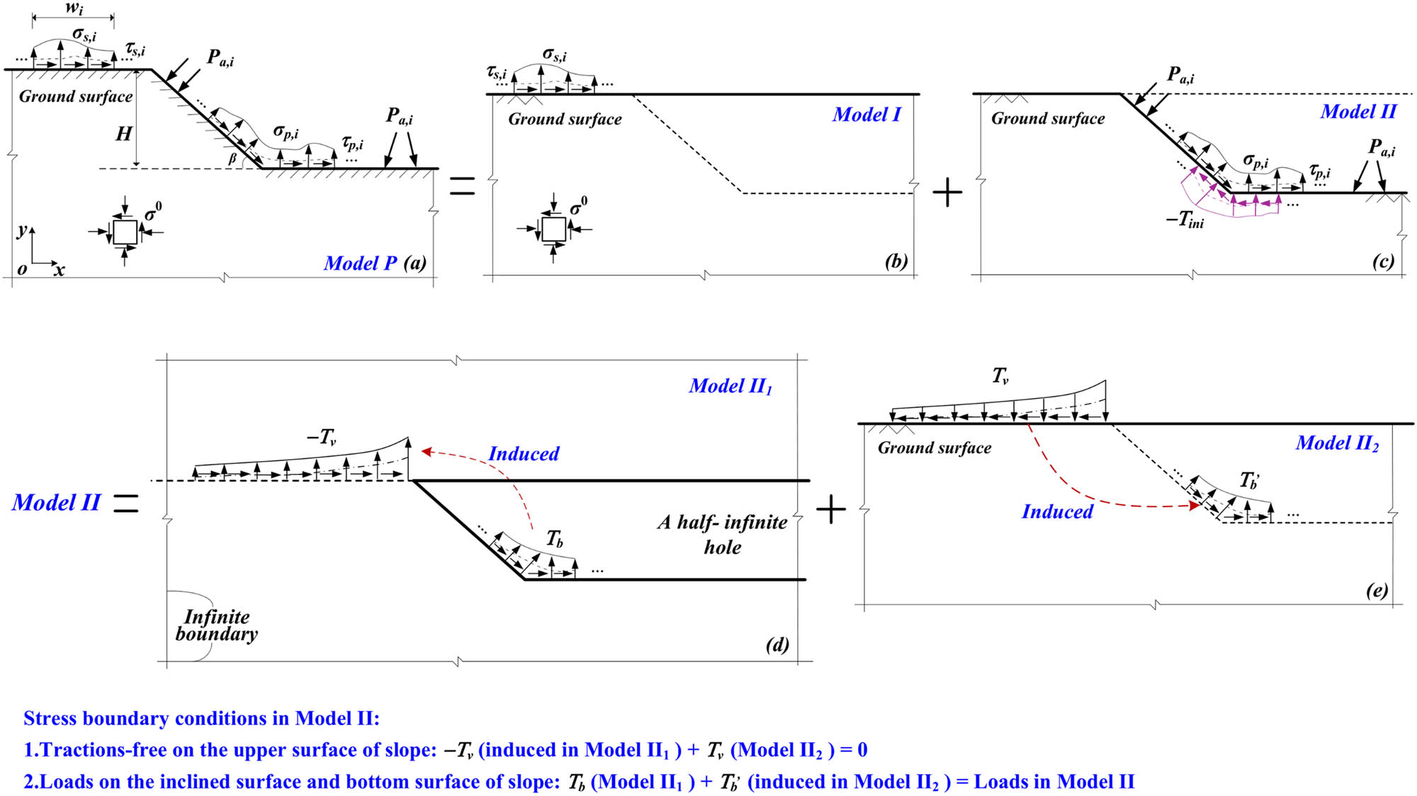
The equivalent model of slope: (a) the prototype model (Model P); (b) a half-plane with surcharges on slope’s crest (Model I); (c) a weightless slope loaded by supporting forces and release stresses (Model II); (d) a half-infinite hole loaded by virtual tractions upon the hole’s boundary in an infinite plane (Model II₁); and (e) a half-plane subjected to virtual tractions along the ground surface (Model II₂).

The current issue’s prototype model, known as Model P, is a slope loaded by the initial earth stress, surcharges, as well as supporting forces, as shown in Figure 1(a). The superposition principle is applicable due to the assumption of linear elasticity with tiny strain herein, which means that the summation of stress solutions in Models I and II is equal to the ultimate stress solution. Model I, shown in Figure 1(b), describes a half-plane that is loaded by surcharges on the crest and initial earth stress within the body. Model II, shown in Figure 1(c), depicts a weightless slope subjected to the release stresses resulting from excavation and the supporting pressures together with any other concentrated forces exerted on the inclined surface and bottom of the slope after excavation. With the aid of the analytical stress solution in a half-plane loaded at its upper surface by concentrated forces (Flamant solution [18]), Model I’s solution is easily accessible. Thus, the crucial step in solving the current problem is to acquire Model II’s analytical stress solution, which can be further equivalent to the superposition of Model II₁ and Model II₂:

Model II₁: depicting an infinite plane containing a half-infinite hole loaded by virtual tractions T b along its boundary, as shown in Figure 1(d), whose solution will be approximated analytically based on the fundamental principle just recently put forth by the authors [19] for solving the elastic stress distribution around a closed convex hole within a half-plane.

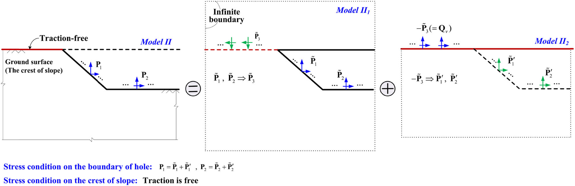
Model II₂: representing a half-plane that is subject to virtual tractions T v along its upper surface (the ground surface), as shown in Figure 1(e), and whose stress solution can also be determined analytically from Flamant solution.

Be aware that Model II’s two sets of virtual tractions are not known in advance, which will be calculated by fulfilling the stress boundary conditions. Since the slope’s crest in Model II is traction-free, the tractions on the line coinciding with the slope’s crest caused by T b acting on the hole’s boundary in Model II₁ must be equal to the virtual tractions’ negative values ( − T v ) , which are applied to the same line in Model II₂. Meanwhile, the total of T b in Model II₁ and the tractions on the hole’s boundary caused by T v in Model II₂ should be exactly equivalent to the actual stress condition in Model II. An appropriate iterative approach can be used to solve for T v and T b , and the specifics will be provided later.

3 Procedures of solution

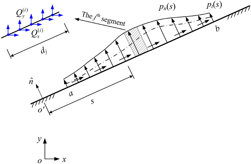
Any sorts of distributed forces, such as virtual tractions, surcharges, and distributed tractions acting on surfaces, can be translated into a sequence of equivalent concentrated forces to simply computation using high-precision numerical integration methods [19]. The stresses created by the distributed forces can thus be identical to those imposed by equivalent concentrated forces. In the subsequent derivation, the Gaussian Quadrature is adopted together with a Legendre polynomial of fifth order [20], which accuracy is suitable for high-precision evaluation of stresses for the problem. The details of transforming tractions to equivalent concentrated forces are described in the Appendix.

3.1 Analytical stress solution for Model I

Model I refers to a pure half-plane loaded by the initial earth stress and surcharge loads upon its upper surface (the same as the slope’s crest), as illustrated in Figure 1(b). The region loaded by the surcharge loads is divided into several segments that are grouped according to type(i) presented in the Appendix. Consequently, the surcharge loads are represented by equivalent concentrated forces, Q s (Figure 2), acting on the ground surface.

Figure 2

A half-plane loaded by initial earth stress and equivalent concentrated forces upon the ground surface.

The stresses at any point in Model I caused by Q s can be calculated using the analytical stress solutions presented in Appendix:

(1) σ s = R s Q s ,

where the components of the matrix R s are calculated using equation (A2) and σ s denotes the stresses caused by Q s .

The stresses at any position in Model I, given by σ I , are thus equal to the total of those induced by surcharge loads using equation (1) and the initial earth stress σ 0 :

(2) σ I = σ s + σ 0 .

3.2 Analytical approximant stress for Model II₁

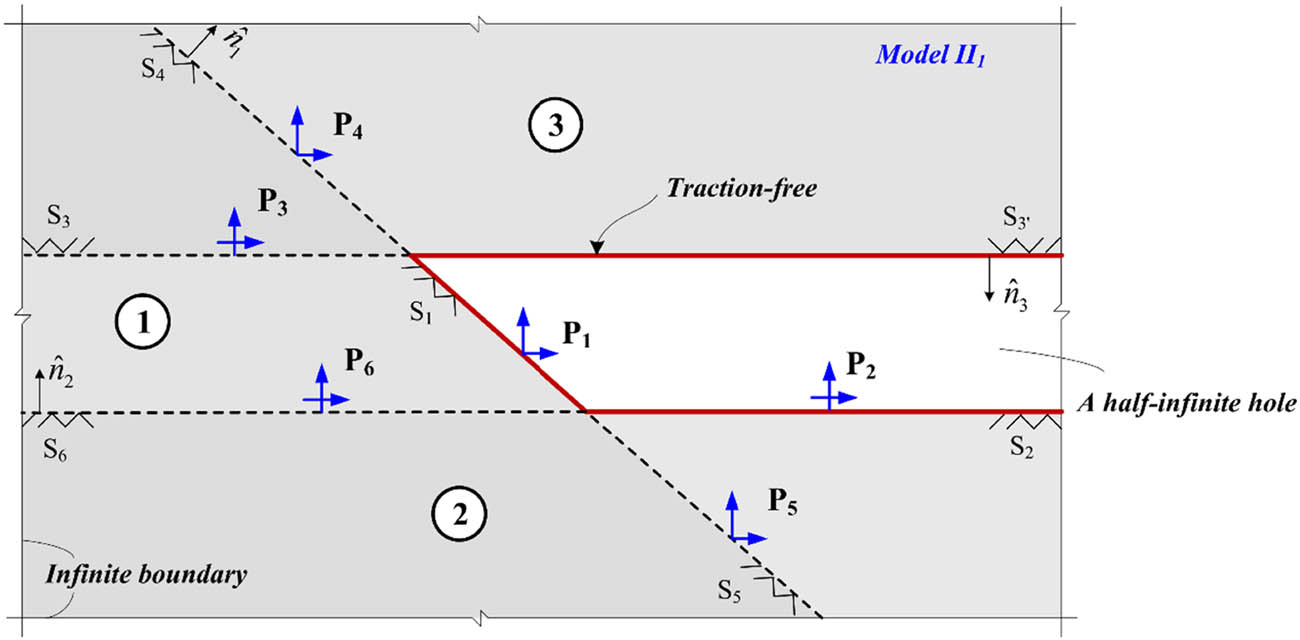
Model II₁ corresponds to a half-infinite hole subjected to virtual tractions T b along its boundary in an infinite plane (Figure 1(d)), whose stresses can be approximated analytically.

The half-infinite hole’s outer region can be considered as the union of three half-planes, each of which corresponds to a specific side of the hole. Consequently, provided that the tractions or the equivalent concentrated forces are known, stresses in the hole’s outer region are the same as those that correspond to a particular half-plane, which can be determined using the Flamant solution. Yet, it is not known beforehand what the tractions will be applied to the half-plane’s outer surfaces that is contained within the adjacent half-plane. Thus, an iterative approach should be used, where the tractions can be initially assumed, typically as zero, and then be updated repeatedly until convergence is achieved to the required degree of accuracy.

It can be seen from Figure 3 that the half-infinite hole’s outer region can be separated into three half-planes by its three sides and their extensions, which are denoted by symbols “①”, “②”, and “③”. The outer surface of the half-plane ① consists of the left external surface S 4 , the side of the hole S 1 , and the right external surface S 5 . The upper surface of the half-plane ② is composed of the hole’s side S 2 and the external surface S 6 . The upper surface of the half-plane ③ consists of the side of the hole S 3 ' and the external surface S 3 .

Figure 3

A half-infinite hole subjected to equivalent concentrated forces in an infinite plane.

The surfaces S 1 , S 2 , S 3 , S 4 , S 5 , and S 6 are assumed to be segmented into many parts. The number of segments of S 2 , S 3 , S 4 , S 5 , and S 6 should be sufficient to limit the error induced by discretization because of stress concentration that exists near the hole’s corner. Type(ii) described in Appendix is suggested as the arrangement for these segments. On contrast, the segments of S 1 can be arranged in type(i) presented in the Appendix.

Therefore, as presented in the Appendix, the distributed tractions applied along surfaces S 1 , S 2 , S 3 , S 4 , S 5 , and S 6 are represented by equivalent concentrated forces P 1 , P 2 , P 3 , P 4 , P 5 , and P 6 , respectively. Concentrated forces are assumed to be applied on the surfaces S 1 and S 2 , if any, these concentrated forces can be added to the equivalent concentrated ones acting at the closest Gaussian points corresponding. Since the Gaussian points are much more densely distributed over the region covering the concentrated forces, such simplification would not lead to unacceptable computation errors.

Now considering the half-plane ③, its external surface S 3 lies within the half-plane ①. It should be noted that the surface S 3 ' is always traction-free and can thus be excluded from consideration. Therefore, by utilizing equation (A12) in the Appendix, along with the superposition principle, P 3 that are applied upon S 3 can be expressed as follows:

(3) P 3 = A 3 , 1 P 1 + A 3 , 4 P 4 + A 3 , 5 P 5 ,

where the components of the matrices A 3 , 1 , A 3 , 4 , and A 3 , 5 are calculated using equation (A12) in the Appendix.

Similarly, the equivalent concentrated forces P 4 , P 5 , and P 6 can be written in the same format as equation(3), namely

(4) P 4 = A 4 , 3 P 3 , P 5 = A 5 , 2 P 2 + A 5 , 6 P 6 , P 6 = A 6 , 1 P 1 + A 6 , 4 P 4 + A 6 , 5 P 5 .

Therefore, once virtual tractions T b are given, that is, the values of P 1 and P 2 are known, it is possible to compute the values of P 3 , P 4 , P 5 , and P 6 using an iterative process within a reasonable tolerance.

The first modified values of P 3 , P 4 , P 5 , and P 6 can be computed using equations (3) and (4), with the initial values of P 3 , P 4 , P 5 , and P 6 being assumed to be zero. The process above is continued until convergence is reached when the maximum difference in values between the two adjacent steps is within an acceptable tolerance by substituting these values into the right side of equations (3) and (4). Following are the steps involved in iteration:

Step 1 : P 3 ( 1 ) = P 4 ( 1 ) = P 5 ( 1 ) = P 6 ( 1 ) = 0 ⇒ P 3 ( 2 ) , P 4 ( 2 ) , P 5 ( 2 ) , P 6 ( 2 ) Step 2 : P 3 ( 2 ) , P 4 ( 2 ) , P 5 ( 2 ) , P 6 ( 2 ) ⇒ P 3 ( 3 ) , P 4 ( 3 ) , P 5 ( 3 ) , P 6 ( 3 ) ⋮ Step k : P 3 ( k ) , P 4 ( k ) , P 5 ( k ) , P 6 ( k ) ⇒ P 3 ( k + 1 ) , P 4 ( k + 1 ) , P 5 ( k + 1 ) , P 6 ( k + 1 ) .

The stresses at a point in Model II₁ after the half-plane including that point has been identified can be calculated using equation (A8) in the Appendix using the convergent values of P 3 , P 4 , P 5 , and P 6 .

3.3 Analytical stress solutions for Model II₂

Model II₂ represents a half-plane without a hole loaded by T v upon its upper surface (Figure 1(e)). The loading region is composed of a number of segments, which are suggested to be arranged in type(ii) presented in the Appendix. Thus, T v can be denoted by equivalent concentrated forces acting at Gaussian points along the slope’s crest, represented by Q v , as depicted in Figure 4.

Figure 4

A pure half-plane loaded by equivalent concentrated forces upon its upper surface.

The stresses in Model II₂ induced by Q v , represented by σ II 1 , can thus be calculated utilizing analytical stress solutions given in the Appendix:

(5) σ II 1 = R v ⋅ Q v ,

where the components of the matrix R v are calculated using equation (A2).

3.4 Iterative process for computing stresses in Model II

Virtual tractions T b and T v in Models II₁ and II₂, respectively, are unknown beforehand in the above derivation, whose values can be obtained by an iterative process with negligible residual errors. The virtual tractions T b corresponding to equivalent concentrated forces Q b consist of P ˜ 1 and P ˜ 2 acting on the hole’s sides S 1 and S 2 , respectively; and T v are represented by Q v , which are identical to − P ˜ 3 acting along the crest of the slope S 3 , as shown in Figure 5. The iteration process is outlined in the following.

Figure 5

Schematic diagram of the iterative calculation.

Assuming the initial values of P ˜ 1 and P ˜ 2 are equal to P 1 and P 2 , respectively, which refer to the equivalent concentrated forces transformed by the tractions induced by the summation of concentrated forces, supporting pressure, and the release stresses, along the hole’s sides S 1 and S 2 in Model II, respectively. The values of P ˜ 3 can then be calculated using equation (3) in Model II₁.

The negative values of P ˜ 3 are obtained, that is, − P ˜ 3 , which are acted on the same region in Model II₂ by satisfying the stress condition on the slope’s crest in Model II. The values of P ˜ 1 ′ and P ˜ 2 ′ acting on S 1 and S 2 , respectively, can be determined using equation (A12) in Model II₂.

Subsequently, by fulfilling the stress condition of the hole’s boundary in Model II, the first modified values of P ˜ 1 and P ˜ 2 can be computed, that is, P 1 = P ˜ 1 + P ˜ 1 ′ and P 2 = P ˜ 2 + P ˜ 2 ′ .

The above procedure is repeated by substituting these values of P ˜ 1 and P ˜ 2 into the above three steps until convergence is achieved, which is determined by the maximum difference in values of P ˜ 1 and P ˜ 2 between the two adjacent iterations being within an acceptable tolerance. Schematically, the process described above is as follows:

Step 1 : P ˜ 1 = P 1 , P ˜ 2 = P 2 ⇒ P ˜ 3 ( Models II 1 )

Step 2 : − P ˜ 3 ⇒ P ˜ 1 ′ , P ˜ 2 ′ ( Models II 2 )

Step 3: P ˜ 1 = P 1 − P ˜ 1 ′ , P ˜ 2 = P 2 − P ˜ 2 ′ ⇒ P ˜ 3 ( Models II 1 ) .

Repeating Steps 2 to 3 until convergence is achieved.

With the convergent values of P ˜ 1 , P ˜ 2 , and P ˜ 3 being obtained, the final stresses at any location within the slope are computed by superimposing the stresses calculated in Models I, II₁, and II₂.

4 Example study and comparison

A vertical slope with a height of H = 10 m is subjected to surcharge loads along its upper surface with a loading width of w = 10 m, as shown in Figure 6(a). The initial earth stress is composed of the vertical and horizontal stresses, with respective values of γ h i and ν γ h i / ( 1 − ν ) , where h i , γ , and ν are the vertical distance from the point considered to the ground surface, the unit weight, and the Poisson’s ratio, respectively. The parameters related to Gaussian points are given in Figure 6. The contour plot of the stress σ y within the slope is depicted in Figure 7.

$Figure 6 A slope with a slope angle of 90° subjected to surcharge loads and initial earth stress. σ s {\sigma }_{s} = 100 kPa, γ \gamma = 20 kN/m3, ν \nu = 0.33). (a) The initial calculation model. (b) The calculation model in ANSYS. (c) The framework in the computation performed in ANSYS.$

Figure 6

A slope with a slope angle of 90° subjected to surcharge loads and initial earth stress. σ s = 100 kPa, γ = 20 kN/m³, ν = 0.33). (a) The initial calculation model. (b) The calculation model in ANSYS. (c) The framework in the computation performed in ANSYS.

Figure 7

Comparisons of contour plots of stress σ _y within slope between the present method and FEM (the unit of stress is kPa).

The FEM is employed in this case for comparison. As shown in Figure 6(b), the calculation model is 40 m high and 70 m long in the X-direction, and a total of 18,571 PLANE 42 elements are generated using the commercial FEM package (ANSYS 15.0). The model’ boundary is outside the affected region by slope excavation. Vertical and horizontal constraints were imposed on the slope’s vertical and horizontal-bottom boundaries, respectively. It can be demonstrated from Figure 7 that the results obtained by the proposed method agree well with those by the FEM, with the exception of a tiny discrepancy existing in the vicinity of the slope toe. Meanwhile, the present approach demonstrates a higher stress concentration, whereas the FEM shows a considerably lower stress concentration despite using a huge number of meshes.

To examine the specifics of stress concentration around the slope toe, the stress diagrams are scaled 10 times, 10² times, and 10⁴ times consecutively, with the horizontal lengths of 10⁻³ H, 10⁻⁵ H, and 10⁻¹⁰ H, respectively, as depicted in Figure 8. Figure 8 illustrates that the stress level measured near the slope toe grows as the diagram’s dimension reduces, while the geometric properties of the stress concentration are almost the same. Additionally, it is demonstrated that the proposed method can predict the stresses in the vicinity of the slope toe, even in the region nearby the slope toe in the range of 10⁻¹¹ H to 10⁻¹⁰ H, which can rarely be obtained using the FEM due to computer capacity and computation time constraints.

Figure 8

Stress diagram at different scales (the unit of stress is kPa).

The distribution of the principal stresses within the slope is presented in Figure 9, from which high-stress concentration appears near the slope toe. It can be seen from Figure 9(a) that the major principal stresses are always compressive, whose contours near the crest and the bottom of the slope are distributed nearly in layers. In contrast, the contours become curves near the inclined surface and the slope toe. From Figure 9(b), the minor principal stresses are also mostly compressive, except for those at the bottom and the region outside the loading region of surcharge loads on the crest of the slope. In the region of the bottom of the slope at a certain distance from the slope toe, the contours are almost horizontal and distributed in the form of layers.

$Figure 9 Contour plots of principal stresses within slope subjected to surcharge loads: (a) σ 1 / γ H {\sigma }_{1}/\gamma H and (b) σ 3 / γ H {\sigma }_{3}/\gamma H .$

Figure 9

Contour plots of principal stresses within slope subjected to surcharge loads: (a) σ 1 / γ H and (b) σ 3 / γ H .

It is assumed to be supported by uniform pressure along the slope’s vertical surface to investigate the effect of supporting forces on the stress distribution within the slope. Contour plots of the major and minor principal stresses within the slope are displayed in Figure 10(a) and 10(b), respectively. It is shown in Figure 10 that the magnitude of stress concentration at the slope toe is smaller than that of the unlined slope (Figure 9). Meanwhile, from Figure 10(b), the tensile stresses occur near the bottom of the slope, the values of which are lower than those in Figure 10(b). As a whole, supporting forces have a remarkable effect on the stress field within the slope, and the present method can provide a theoretical tool for the design of slope reinforcements.

$Figure 10 Contour plots of stresses within the slope supported by uniform pressure along the slope surface: (a) σ 1 / γ H {\sigma }_{1}/\gamma H and (b) σ 3 / γ H {\sigma }_{3}/\gamma H .$

Figure 10

Contour plots of stresses within the slope supported by uniform pressure along the slope surface: (a) σ 1 / γ H and (b) σ 3 / γ H .

5 Application

A slope with a height of H = 10 m is considered, as shown in Figure 11, with an inclination of chosen as 10, 20, 30, 40, 50, 60, 70, 80, and 90°. The unit weight γ is 20 kN/m³, and the Poisson’s ratio ν is 0.33. The initial earth stress considered herein consists of the vertical and horizontal stresses with respective values of γ h i and ν γ h i / ( 1 − ν ) . The normalized stresses σ x ⁎ / γ H , σ y ⁎ / γ H , and τ x y ⁎ / γ H , representing the stresses solely induced by excavation, along several vertical lines in the slope, are presented in Figure 12. Therefore, the actual stresses at any point within the slope, denoted by σ act , can be obtained by the summation of these stresses and the earth stress, that is,

(6) σ act = σ x ⁎ σ y ⁎ τ x y ⁎ + σ x 0 σ y 0 0 ,

where σ act = ( σ x act , σ y act , τ x y act ) T , σ x 0 = ν / ( 1 − ν ) γ h , and σ y 0 = γ h , in which h is the vertical distance from the point under consideration to the slope’s surface.

Figure 11

Geometry of a typical slope.

$Figure 12 Values of σ x ⁎ / γ H {\sigma }_{x}^{\ast }/\gamma H , σ y ⁎ / γ H {\sigma }_{y}^{\ast }/\gamma H , and τ x y ⁎ / γ H {\tau }_{xy}^{\ast }/\gamma H along seven lines (Figure 11). (a) Line 1, (b) Line 2, (c) Line 3, (d) Line 4, (e) Line 5, (f) Line 6, and (g) Line 7.$

Figure 12

Values of σ x ⁎ / γ H , σ y ⁎ / γ H , and τ x y ⁎ / γ H along seven lines (Figure 11). (a) Line 1, (b) Line 2, (c) Line 3, (d) Line 4, (e) Line 5, (f) Line 6, and (g) Line 7.

It can be seen from Figure 12 that the inclination angle has a remarkable effect on the stress distribution within the slope; the normalized stresses σ x ⁎ / γ H , σ y ⁎ / γ H , and τ x y ⁎ / γ H increase with the increase of the depth and increase with the increase of the inclination angle.

It is illustrated from Figure 12(a) (Line 1, vertical line at a horizontal distance of H from the slope crown) that the normalized stresses σ x ⁎ / γ H and τ x y ⁎ / γ H convert from tensile to compressive with the increase of the depth, while the normalized stress σ y ⁎ / γ H is always tensile. The normalized stresses σ x ⁎ / γ H , σ y ⁎ / γ H , and τ x y ⁎ / γ H increase as the slope becomes steeper. It can be seen from Figure 12(c) (Line 3, vertical line through the slope crown) that the normalized stress σ x ⁎ / γ H near the apex of the slope decreases gradually with an increase in the inclination angle, while the normalized stress σ y ⁎ / γ H increases. It must be noted that most of the tensile stresses in these cases could be eliminated on superposition of the initial earth stress.

It can be illustrated from Figure 12(e) (Line 5, vertical line through the slope toe) that high-stress concentration appears at the slope toe when the inclination angle is more than 50°, the magnitude of which increases as the inclination angle increases. When the depth is more than 4H, the curves of the normalized stresses σ x ⁎ / γ H , σ y ⁎ / γ H , and τ x y ⁎ / γ H nearly remain constant.

For the stresses at some distance from the slope toe (Figure 12(g), Line 7), the normalized stresses σ x ⁎ / γ H and τ x y ⁎ / γ H increase significantly with the depth increasing from 0 to 2.5H and then slightly from 2.5H to 4.5H, below which the normalized stresses remain constant. In contrast, the normalized stress σ y ⁎ / γ H increases as the depth increases. For slopes of all inclination angles, when the depth is higher than 3H, σ y ⁎ / γ H increases in direct proportion to the depth.

For the sake of practical application, choosing a series of stand slopes with various values of inclination angles, contour plots of stresses are developed for the normalized stresses σ 1 / γ H (major principal stress), σ 3 / γ H (minor principal stress), and τ max / γ H (maximum shear stress), and vectors of major and minor principal stresses are presented in Figures 13–21.

Figure 13

Stress distribution within a slope of the inclination angle of 10°: (a)–(c) contour plots of stresses and (d) vectors of major and minor principal stresses.

Figure 14

Stress distribution within a slope of the inclination angle of 20°: (a)–(c) contour plots of stresses and (d) vectors of major and minor principal stresses.

Figure 15

Stress distribution within a slope of the inclination angle of 30°: (a)–(c) contour plots of stresses and (d) vectors of major and minor principal stresses.

Figure 16

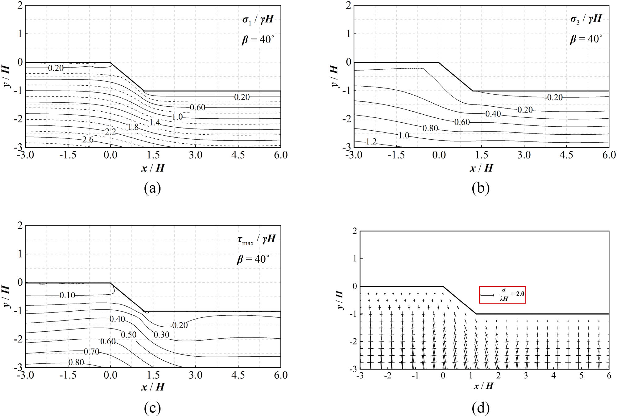
Stress distribution within a slope of the inclination angle of 40°: (a)–(c) contour plots of stresses and (d) vectors of major and minor principal stresses.

Figure 17

Stress distribution within a slope of the inclination angle of 50°: (a)–(c) contour plots of stresses and (d) vectors of major and minor principal stresses.

Figure 18

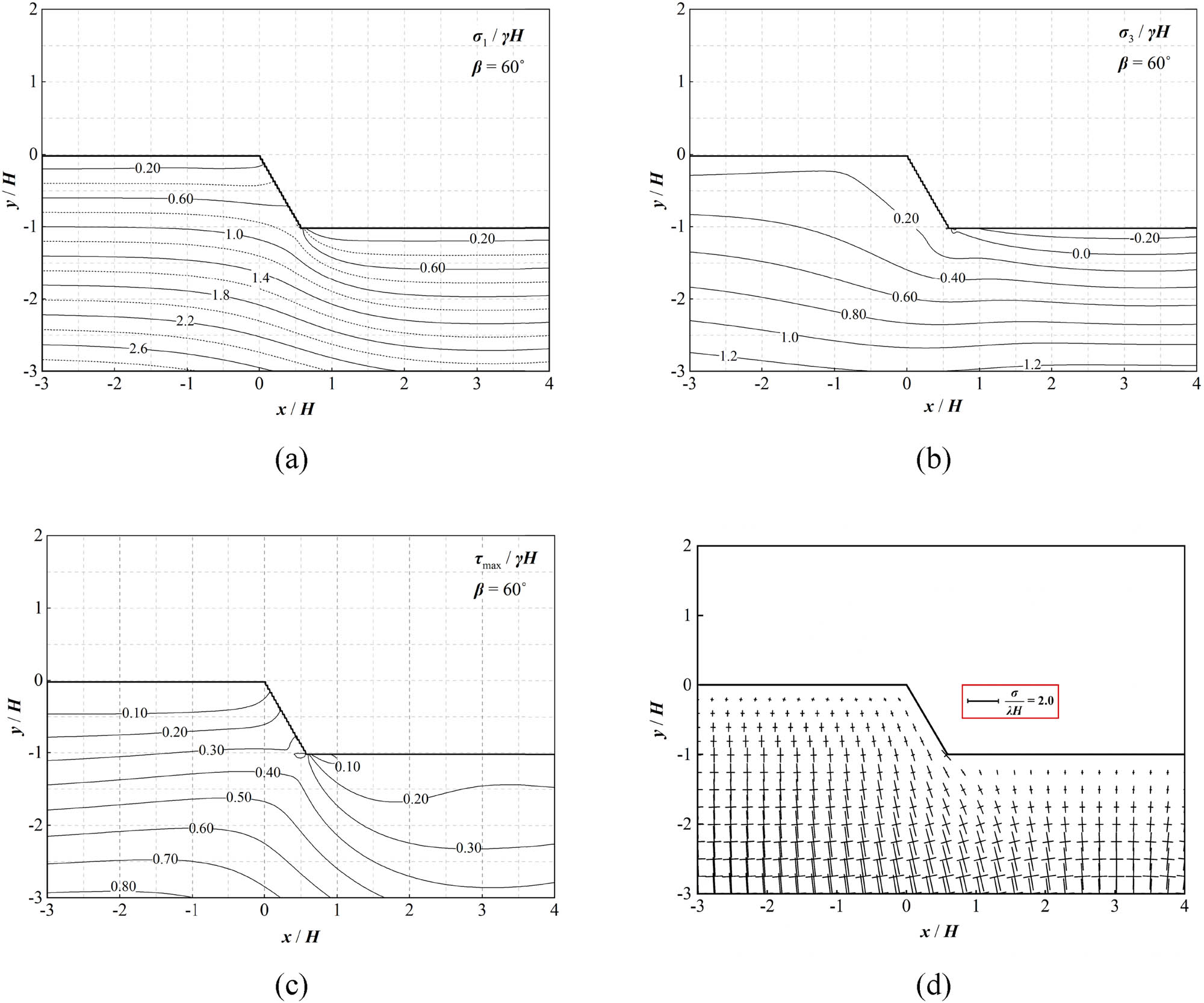
Stress distribution within a slope of the inclination angle of 60°: (a)–(c) contour plots of stresses and (d) vectors of major and minor principal stresses.

Figure 19

Stress distribution within a slope of the inclination angle of 70°: (a)–(c) contour plots of stresses and (d) vectors of major and minor principal stresses.

Figure 20

Stress distribution within a slope of the inclination angle of 80°: (a)–(c) contour plots of stresses and (d) vectors of major and minor principal stresses.

Figure 21

Stress distribution within a slope of the inclination angle of 90°: (a)–(c) contour plots of stresses and (d) vectors of major and minor principal stresses.

With these contour plots, the stresses at any point within a given slope can be directly obtained. For example, it is required to determine the stresses σ 1 , σ 3 , and τ max at the point (x, y), where x = −11.6 m and y = −28.16 m, within a vertical slope of height H = 20 m. Poisson’s ratio ν is equal to 0.33, and the unit weight γ is equal to 25 kN/m³. Corresponding to x = −0.581H and y = −1.408H, Figure 21 gives σ 1 / γ H = 1.331, σ 3 / γ H = 0.415, and τ max / γ H = 0.458. Then, σ 1 = 665.5 kPa, σ 3 = 207.5 kPa, and τ max = 229.0 kPa.

For a standard slope with arbitrary inclination, we can choose two standard slopes with inclinations slightly larger and lesser than that of the specific slope, and the required stresses can be obtained by linear interpolation from the results of the two standard slopes. It has been known that in normal situations with a moderate magnitude of horizontal earth stresses, the effect of horizontal earth stresses on stresses within the slope is insignificant from practical viewpoints. Thus, the effect of the value of Poisson’s ratio ν can also be neglected, and these diagrams would have general applications for roughly estimating elastic stress distribution within a slope of any height, inclination, and unit weight as well. Besides, it should be noted that the pore-water pressure or any form of water content is not considered in the derivation of the proposed solution.

6 Conclusion

In this article, approximate analytic solutions for elastic stresses within a slope subjected to general loading conditions are provided. Surcharge loads and other supporting forces, such as pressure and concentrated forces, can be incorporated into the solution, which can sufficiently approach the analytical solutions with a much high degree of precision. The procedure of the solution is straightforward and easily implementable into a computer program.

The example’s results demonstrate that the stresses calculated using the present method and the FEM are in good agreement. In addition, it is possible to accurately determine the stresses that have not yet been available achieved by any other numerical methods in the region around the proximity of the slope toe, even at distances between 10⁻¹¹ and 10⁻¹⁰ times the slope’s height. The effect of supporting forces on the stress distribution within the slope is also investigated, and the findings demonstrate that supporting forces have an impact on the stress distribution within the slope.

With the present method, contour plots of stresses are presented for nine standard slopes of various inclination angles. The results show that the inclination angle has a remarkable effect on the stress distribution within slope, and the larger the inclination is, the higher the stress concentration near the slope toe is. For a slope with arbitrary inclination, we can choose two standard slopes with inclinations slightly larger and lesser than that of the specific slope, and the required stresses can be obtained by linear interpolation from the results of the two standard slopes. These contour plots of stresses would have general applications for roughly estimating elastic stress distribution within a slope of any height, inclination and unit weight as well.

Acknowledgements

The authors thank the help and guidance from Prof. Kunlin LU of Hefei University of Technology and Prof. Rongzhu LIANG from China University of Geosciences.

Funding information: This research was funded by the National Natural Science Foundation of China (Grant Number 52079121).
Author contributions: The whole manuscript was written and edited by Ping WU, the work herein was guided and rechecked thoroughly by Prof. D.Y. Zhu, and the structure and tongue of this work were assisted by Prof. X.J. Sun. All authors rechecked and approved the final manuscript.
Conflict of interest: The authors declare that they have no known competing financial interests or personal relationships that could have appeared to influence the work reported in this paper.
Ethical approval: The conducted research is not related to either human or animal use.
Data availability statement: The datasets generated during and/or analyzed during the current study are available from the corresponding author on reasonable request.

Appendix

A1 Derivation of equations and illustration of some concepts

A1.1 Analytical stress solution for a half-plane subjected to concentrated forces

In the coordinate system oxy, horizontal and vertical concentrated forces, P x and P y , are applied at a point O ′ on the upper surface of a half-plane (Figure A1). The analytical solution of stresses (only the radial stress is created) in the local polar coordinate system at point A can be expressed based on Flamant’s solution [18].

(A1) σ r = − 2 P x π r cos θ − 2 P y π r sin θ ,

in which r = ( x A − x O ′ ) 2 + ( y A − y O ′ ) 2 , sin θ = ( x A − x O ′ ) / r , and cos θ = ( y A − y O ′ ) / r .

Figure A1

A half-plane loaded by concentrated forces.

In the framework of a unified cartesian coordinate system, equation (A1) can be transformed into

(A2) σ = D P ,

where σ = ( σ x , σ y , τ x y ) T , P = ( P x , P y ) T , and D = − 2 π r cos 3 θ cos θ sin 2 θ cos 2 θ sin θ cos 2 θ sin θ sin 3 θ cos θ sin 2 θ .

The components D depend solely on the specific location of point A, where stresses are to be calculated, in relation to point O ′ , where the concentrated forces are acting, that is

(A3) D = D ( x A , y A , x O ′ , y O ′ ) .

A1.2 Conversion of tractions into equivalent concentrated forces

Given that normal and tangential stresses, p n ( s ) and p t ( s ) , are applied upon the upper surface of a half-plane (Figure A2). The horizontal and vertical tractions, p x and p y , in the x and y directions, respectively, can be written as follows:

(A4) p x p y = N p n p t ,

where N = n x n y n y − n x , n x = cos ( n ˆ , x ) , and n y = cos ( n ˆ , y ) . n ˆ represents the upper surface’s outward normal.

Figure A2

A half-plane under distributed tractions.

The region in the interval ab loaded by the distributed tractions is divided into n segments, each comprising five Gaussian points, sufficiently satisfying the need for high precision, as depicted in Figure A2. Thus, there are a total of m (= 5 ⋅ n ) Gaussian points within ab. The position of the ith Gaussian point, which lies within the jth segment, can be stated as

(A5) s i = a + ζ i d j , i = 1 , 2 , … , m ; j = 1 , 2 , … , n ,

where d j is the length of the jth segment and ζ i indicates the parameter related to where the ith Gaussian point is located. ζ is equivalent to 0.04691, 0.230765, 0.5, 0.769235, and 0.95309, respectively, for each segment’s five Gaussian points [20].

Thus, the distributed traction is substituted with m equivalent concentrated forces acting at Gaussian points within ab. Based on equation (A4) and Gaussian Quadrature theory, equivalent concentrated forces Q x ( i ) and Q y ( i ) acting at the ith Gaussian points within the jth segment are denoted as follows:

(A6) Q x ( i ) Q y ( i ) = g i p x ( i ) p y ( i ) ,

where g i = c i d j and c i represents the coefficient of the Gaussian point. For five Gaussian points of each segment, c is equal to 0.118463, 0.239314, 0.284444, 0.239314, and 0.118463 [20].

The equivalent concentrated forces acting at all of the Gaussian points within ab, represented by Q , are then assembled using equation (A6), that is,

(A7a) Q = G ⋅ p ,

(A7b) Q = ( Q x ( 1 ) , Q y ( 1 ) , Q x ( 2 ) , Q y ( 2 ) , … , Q x ( m ) , Q y ( m ) ) T ,

(A7c) p = ( p x ( 1 ) , p y ( 1 ) , p x ( 2 ) , p y ( 2 ) , … , p x ( m ) , p y ( m ) ) T ,

(A7d) G = g 1 g 1 0 0 0 ⋮ 0 0 0 0 g 2 g 2 0 ⋮ 0 0 0 0 0 0 ⋱ ⋮ 0 0 ⋯ 0 ⋯ 0 ⋯ 0 ⋯ 0 ⋯ 0 ⋮ ⋮ ⋯ g m ⋯ g m .

A1.3 Equivalent concentrated forces on a line within a half-plane loaded by equivalent concentrated forces

Assuming that a half-plane is loaded by distributed tractions with the width s i upon its upper surface. As previously mentioned, the loading zone can be divided into a number of segments with a total of m i Gaussian points (Figure A3). The tractions are therefore identical to the equivalent concentrated forces at all Gaussian points, denoted by Q i .

Figure A3

A half-plane loaded by equivalent concentrated forces upon its upper surface.

The stresses within the half-plane induced by Q i can thus be determined using equation (A2) and the superposition principle

(A8) σ = R i ⋅ Q i ,

where R i = ( D i 1 , D i 2 , ⋯ , D i m i ) , the components of which can be calculated using equation (A2).

Given that a segment s j located within the half-plane with a total of m j Gaussian points, the stresses at the kth Gaussian point on this segment, represented by σ j ( k ) , can thus be computed using equation (A8). Following that, by transforming the stresses into the tractions acting at this Gaussian point, indicated by { p j , x ( k ) , p j , y ( k ) } , we obtain

(A9) p j , x ( k ) p j , y ( k ) = M j σ j ( k ) , k = 1 , 2 , 3 , … , m j ,

where M j = n j , x 0 n j , y 0 n j , y n j , x , n j , x = cos ( n ˆ j , x ) , and n j , y = cos ( n ˆ j , y ) ; in which n ˆ j is the outward normal of the surface where the segment s j lies within.

Substituting equation (A8) into equation (A9) yields

(A10) p j , x ( k ) p j , y ( k ) = M j ⋅ R j i ( k ) ⋅ Q i ,

Thus, the tractions acting at all Gaussian points within the segment s j can be assembled, denoted by p j , that is

(A11) p j = U j , i ⋅ Q i ,

where U j , i = M j ⋅ R j i ( 1 ) M j ⋅ R j i ( 2 ) ⋮ M j ⋅ R j i ( m i ) .

The equivalent concentrated forces acting at all Gaussian points on the segment s j caused by Q i , denoted by Q j , are then written as follows using equation (A7a):

(A12) Q j = A j , i Q i ,

where A j , i = G j ⋅ U j , i .

A1.4 General types of discretization of a line into segments

The area subjected to the distributed tractions should be divided into a number of segments, which are recommended to be arranged in accordance with three types of discretization outlined below, as depicted in Figure A4.

Figure A4

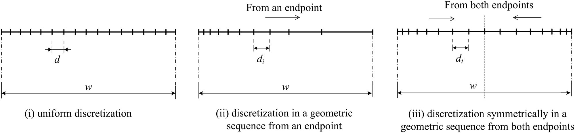
General types of discretization of a line into segments: (i) uniform discretization, (ii) discretization in a geometric sequence from an endpoint, and (iii) discretization symmetrically in a geometric sequence from both endpoints.

Type (i): uniform discretization

The segments of the loading region are discretized uniformly with a length of d .

Type (ii): discretization in a geometric sequence from an endpoint

The region consists of n segments, which are discretized in a geometric sequence from an endpoint of the region. The length of the segment is expressed as

(A13) d i = d 1 ( q ) i − 1 , ( i = 1 , 2 , ⋯ , n ) ,

where d i is the ith segment’s length; q is the geometric sequence’s common ratio.

Type (iii): discretization symmetrically in a geometric sequence from both endpoints

The region is divided into n segments ( n is odd integer). These segments are discretized symmetrically in a geometric sequence from both endpoints of the region, of which the length is expressed as

(A14) d i = d 1 ( q ) i − 1 , i = 1 , 2 , … , n − 1 2 , w − d 1 ( q ) n − i − 1 , i = n − 1 2 , n + 1 2 , … , n ,

where d i is the length of the ith segment and q is the common ratio of the geometric sequence.

References

[1] Wright SG, Kulhawy FH, Duncan JM. Accuracy of equilibrium slope stability analysis. J Soil Mech Found Div J. 1973;99(10):783–91. 10.1061/JSFEAQ.0001933.Search in Google Scholar

[2] Tavenas F, Trak B, Leroueil S. Remarks on the validity of stability analyses. Can Geotech J. 1980;17(1):61–73. 10.1139/t80-006.Search in Google Scholar

[3] Zhu DY, Lee CF, Jiang HD. Generalized framework of limit equilibrium methods for slope stability analysis. Geotechnique. 2003;53(4):377–95. 10.1680/geot.2003.53.4.377.Search in Google Scholar

[4] Zhu DY, Lee CF, Chan DH, Jiang HD. Evaluation of the stability of anchor-reinforced slopes. Can Geotech J. 2005;42(5):1342–9. 10.1139/t05-060.Search in Google Scholar

[5] Cheng H, Zhou X. A novel displacement-based rigorous limit equilibrium method for three-dimensional landslide stability analysis. Can Geotech J. 2015;52(12):2055–66. 10.1139/cgj-2015-0050.Search in Google Scholar

[6] Zienkiewicz OC, Taylor RL, Taylor RL. The finite element method: solid mechanics. Vol. 2. Butterworth-heinemann; 2000.Search in Google Scholar

[7] Matsui T, San K. Finite element slope stability analysis by shear strength reduction technique. Soils Found. 1992;32(1):59–70. 10.3208/sandf1972.32.59.Search in Google Scholar

[8] Kim JY, Lee SR. An improved search strategy for the critical slip surface using finite element stress fields. Comput Geotech. 1997;21(4):295–313. 10.1016/S0266-352X(97)00027-X.Search in Google Scholar

[9] Liu S, Su Z, Li M, Shao L. Slope stability analysis using elastic finite element stress fields. Eng Geol. 2020;273:105673. 10.1016/j.enggeo.2020.105673.Search in Google Scholar

[10] Yang Y, Wu W, Zheng H. Searching for critical slip surfaces of slopes using stress fields by numerical manifold method. J Rock Mech Geotech Eng. 2020;12(6):1313–25. 10.1016/j.jrmge.2020.03.006.Search in Google Scholar

[11] Brebbia CA. The boundary element method for engineers. Plymouth: Pentech Press; 1978.Search in Google Scholar

[12] Martel SJ, Muller JR. A two-dimensional boundary element method for calculating elastic gravitational stresses in slopes. Pure Appl Geophys. 2000;157(6):989–1007. 10.1007/s000240050014.Search in Google Scholar

[13] Ostanin IA, Mogilevskaya SG, Labuz JF, Napier J. Complex variables boundary element method for elasticity problems with constant body force. Eng Anal Bound Elem. 2011;35(4):623–30. 10.1016/j.enganabound.2010.11.008.Search in Google Scholar

[14] Silvestri V, Tabib C. Exact determination of gravity stresses in finite elastic slopes: Part I. Theoretical considerations. Can Geotech J. 1983;20(1):47–54. 10.1139/t83-005.Search in Google Scholar

[15] Savage WZ. Gravity-induced stresses in finite slopes. Int J Rock Mech Min Sci Geomech Abstr.; 1994. p. 471–83. 10.1016/0148-9062(94)90150-3.Search in Google Scholar

[16] Hasebe N, Wang XF. Irregular elastic half-plane gravity problem. Int J Rock Mech Min. 2003;40(6):863–75. 10.1016/S1365-1609(03)00054-6.Search in Google Scholar

[17] Jia X, Lu A, Cai H, Ma Y. An analytical method for solving gravity-induced stresses in slope. Appl Math Model. 2021;98:665–79. 10.1016/j.apm.2021.06.004.Search in Google Scholar

[18] Barber JR. Elasticity. Dordrecht: Kluwer Academic Publishers; 2002.Search in Google Scholar

[19] Zhu DY, Wu P. Asymptotically analytical solution of elastic stress for convex polygonal holes in an infinite plane under various loading conditions. Acta Mech. 2021;232(10):3957–75. 10.1007/s00707-021-03040-2.Search in Google Scholar

[20] Burden RL, Faires JD. Numerical analysis. 9th edn. Boston: Brooks/Cole Cencag Learning; 2011.Search in Google Scholar

Received: 2023-02-03

Revised: 2023-05-25

Accepted: 2023-05-25

Published Online: 2023-06-14

This work is licensed under the Creative Commons Attribution 4.0 International License.

Articles in the same Issue

https://doi.org/10.1515/arh-2022-0156

Keywords for this article

semi-analytical stress solution; half-infinite hole; slope; half-plane

Creative Commons

BY 4.0

Semi-analytical method for solving stresses in slope under general loading conditions

Article

Abstract

1 Introduction

2 Fundamentals

3 Procedures of solution

3.1 Analytical stress solution for Model I

3.2 Analytical approximant stress for Model II1

3.3 Analytical stress solutions for Model II2

3.4 Iterative process for computing stresses in Model II

4 Example study and comparison

5 Application

6 Conclusion

Acknowledgements

Appendix

A1 Derivation of equations and illustration of some concepts

A1.1 Analytical stress solution for a half-plane subjected to concentrated forces

A1.2 Conversion of tractions into equivalent concentrated forces

A1.3 Equivalent concentrated forces on a line within a half-plane loaded by equivalent concentrated forces

A1.4 General types of discretization of a line into segments

References

Articles in the same Issue

Articles in the same Issue

Articles in the same Issue

3.2 Analytical approximant stress for Model II₁

3.3 Analytical stress solutions for Model II₂