On some dense sets in the space of dynamical systems

1 Introduction

The notion of chaos first appeared in 1975 in [8]. Since then, many different and non-equivalent definitions of chaos have been formulated. The survey of these concepts and an indication of their mutual dependence one can find, for example, in [9,13]. It is worth noting that some research also refers to the local properties of the dynamical system. For example, proposals for points of chaos (points around which the chaos focuses, e.g., [2,10,11]) have recently appeared. Of course, in many cases, these issues are naturally related to entropy. We will consider points focusing entropy, chaos, and distributional chaos of periodic dynamical systems. It is not difficult to notice the independence of these concepts. We aim to explore it more deeply in this article. For this purpose, we will use the metric space of all periodic dynamical systems acting in the unit interval. We will prove that each of the sets of systems having a point that has exactly one of the aforementioned properties, and a set of systems having a point that has all of them are dense in the considered space. The natural consequence of this is the remark that each of these sets has an empty interior.

We use standard symbols and notations. By N + , N 0 , R , I , and X we denote the set of all positive integers, non-negative integers, real numbers, interval [ 0 , 1 ] , and non-degenerate compact subinterval of I , respectively. To simplify the notation, we use the same letters R , I , and X for metric spaces equipped with the natural metric. For closed (right hand-open, etc.) intervals, we use the standard notion [ a , b ] ( [ a , b ) , etc.). Moreover, symbol 〚 a , b 〛 stands for a set [ a , b ] ∩ N 0 . By log , we mean the logarithm with the base 2. Cardinality of the set A is denoted by card ( A ) . Now let x ∈ X , r > 0 . Symbol B ( x , r ) ( B ¯ ( x , r ) ) stands for an open (closed) ball in space X with centre at x and radius r . In this way, we avoid the intersection of type ( x − r , x + r ) ∩ X . By C ( X ) , we denote the set of all continuous functions f : X → X , and we treat it as a metric space with a uniform metric d , given by a formula d ( f , g ) = min { 1 , sup { ∣ f ( x ) − g ( x ) ∣ : x ∈ X } } for f , g ∈ C ( X ) .

According to the assumption mentioned earlier, we focus on local properties of dynamical systems consisting of functions from C ( X ) . The definitions and theorems are taken from [1,3,5].

Consider f ∈ C ( X ) . By f − 1 , we denote the inverse function or preimage, depending on the context. Let A , B ⊂ X . We say that a set A f-covers set B (briefly A → f B ) if B ⊂ f ( A ) . The set A ⊂ X is called f -invariant if f ( A ) ⊂ A .

A non-autonomous dynamical system is a pair ( X , ( f 1 , ∞ ) ) , where ( f 1 , ∞ ) is a sequence of continuous self-maps { f j } j = 1 ∞ defined on X . For simplicity, we denote it by ( f 1 , ∞ ) or ( f 1 , f 2 , … ) . If f j = f for all j ∈ N + , the system is called an autonomous dynamical system and is denoted by ( f ) .

We say that a dynamical system ( f 1 , ∞ ) = { f j } j = 1 ∞ is periodic if there exists a positive integer k ∈ N + , called a period of the system, such that f j = f j mod k if j mod k ≠ 0 , and f j = f k otherwise. By P ( f 1 , ∞ ) , we denote the set of all periods of the system ( f 1 , ∞ ) . If k ∈ P ( f 1 , ∞ ) , then we sometimes write ( f 1 , … , f k ) instead of ( f 1 , ∞ ) . Let us note some agreements related to notations and some properties of dynamical systems [5]. Consider a dynamical system ( f 1 , ∞ ) and j , m ∈ N + . Then f j 0 is the identity function (we write id X ) and, moreover, let f j m = f j + m − 1 ∘ f j + m − 2 ∘ ⋯ ∘ f j + 1 ∘ f j . In the case of an autonomous system ( f ) , we write briefly f m instead of f j m . By ( f 1 , ∞ m ) , we denote a sequence { f i m + 1 m } i = 0 ∞ = ( f 1 m , f m + 1 m , f 2 m + 1 m , … ) . If m ∈ P ( f 1 , ∞ ) and a ∈ N + , then f 1 a ⋅ m = ( f 1 m ) a and ( f 1 , ∞ m ) = ( f 1 m ) . Now we note definitions and symbols introduced in [12], which will be useful in this article. Let ( f 1 , ∞ ) be a periodic non-autonomous dynamical system. Then each system ( ψ ) such that ψ = f 1 k , k ∈ P ( f 1 , ∞ ) , is called a dynamical system generated by ( f 1 , ∞ ) . The system ( f 1 , ∞ ) is called a periodic generator of ( ψ ) . By PG ( ψ ) , we denote the set of all periodic generators of the system ( ψ ) .

Let x 0 ∈ X . A point x 0 is called a fixed point of function f (briefly x 0 ∈ Fix ( f ) ) if x 0 = f ( x 0 ) and similarly x 0 is called a fixed point of the system ( f 1 , ∞ ) (briefly x 0 ∈ Fix ( f 1 , ∞ ) ) if f j ( x 0 ) = x 0 for j ∈ N + . We say that x 0 is a periodic point with period n ∈ N + of the system ( f 1 , ∞ ) if f 1 k n ( x 0 ) = x 0 for k ∈ N + . The set of all periodic points with period n of the system ( f 1 , ∞ ) is denoted by Per n ( f 1 , ∞ ) . Put Per ( f 1 , ∞ ) = ⋃ n = 1 ∞ Per n ( f 1 , ∞ ) . Let ( f 1 , ∞ ) = { f j } j = 1 ∞ , ( g 1 , ∞ ) = { g j } j = 1 ∞ be a periodic non-autonomous dynamical systems defined on X , consisting of continuous functions. Put ρ ( f 1 , ∞ , g 1 , ∞ ) = sup { d ( f j , g j ) : j ∈ N + } . Then ρ is a metric in the space of all periodic non-autonomous dynamical systems defined on X .

By the symbol U X , we denote the metric space of dynamical systems consisting of continuous functions defined on X with the metric ρ . By U X p , we will denote its subspace consisting of periodic systems of any period.

The entropy of dynamical systems is one of the basic concepts used in this article (and in many articles connected with dynamical systems). We formulate the definition of entropy following [5]. Let us consider a dynamical system ( X , ( f 1 , ∞ ) ) . Fix n ∈ N + , ε > 0 , and let Y ⊂ X . We say that a set E ⊆ Y is ( n , ε ) -separated in Y if for any distinct points x , y ∈ E there exists j ∈ 〚 0 , n − 1 〛 such that ∣ f 1 j ( x ) − f 1 j ( y ) ∣ > ε . By s n ( f 1 , ∞ , Y , ε ) , we denote the maximal cardinality of ( n , ε ) -separated set in Y . If Y = X , then we note s n ( f 1 , ∞ , ε ) . The topological entropy of a system ( X , ( f 1 , ∞ ) ) on Y ⊂ X is the number h ( f 1 , ∞ , Y ) = lim ε → 0 limsup n → ∞ 1 n log s n ( f 1 , ∞ , Y , ε ) . If Y = X , then we use the symbol h ( f 1 , ∞ ) . In the case of an autonomous system ( f ) , we briefly write h ( f , Y ) or h ( f ) . In many cases, we use the results from [5], calling them lemmas.

Now, based on [1,3], we write down useful statements.

Let us now note the lemma (the proof is obvious) and the corollary that follows from it.

Next definition is based on [6,15]. In the first of these papers, the full entropy point was defined for dynamical systems consisting of homeomorphisms with positive entropy. In [6], the homeomorphism assumption was abandoned. The definition adopted in this article allows us to consider a wide class of functions.

Let ( f 1 , ∞ ) = { f j } j = 1 ∞ ∈ U X . We say that x 0 ∈ X is a point focusing entropy of a system ( f 1 , ∞ ) if for any open neighbourhood U of x 0 equality h ( f 1 , ∞ , U ) = h ( f 1 , ∞ ) holds. Now let us prove the useful theorem.

During the study of the local aspects of dynamical systems, the chaotic points were analyzed, among others. In this article, we base on concepts from [10–12]. Let ( f 1 , ∞ ) be a dynamical system on X and x 0 ∈ Per ( f 1 , ∞ ) . By W ( x 0 , f 1 , ∞ ) , we denote the set of all points t ∈ X such that there exist sequences { y n } n = 1 ∞ ⊂ X and { k n } n = 1 ∞ ⊂ N 0 such that y n → x 0 and f 1 k n ( y n ) = t . Let x 0 ∈ Per ( f 1 , ∞ ) . A point t ∈ X is called an ( x 0 , f 1 , ∞ ) -homoclinic point if x 0 ≠ t ∈ W ( x 0 , f 1 , ∞ ) and x 0 is a limit of { f 1 m k ( t ) } k = 0 ∞ for some sequence of positive integers { m k } k = 0 ∞ .

We say that a point x 0 is a chaotic point of a system ( f 1 , ∞ ) if for each neighbourhood of x 0 , there exists an ( x 0 , f 1 , ∞ ) -homoclinic point.

In 1994, Schweizer and Smítal have introduced the concept of distributional chaos [14]. Eighteen years later, Dvořáková [4] generalized this notion for the case of non-autonomous dynamical systems. This article is based on this concept. Due to restriction of our considerations to X , the following definitions also are formulated only for this space.

Let ( f 1 , ∞ ) be a dynamical system on X , fix t > 0 and x , y ∈ X . Consider the functions given by the formulas:

Let x , y ∈ X . We say that a pair ( x , y ) is distributionally chaotic of type 1 for a dynamical system ( f 1 , ∞ ) if Φ x , y ∗ ( f 1 , ∞ ) ( t ) = 1 for any t > 0 and there exists t 0 > 0 such that Φ x , y ( f 1 , ∞ ) ( t 0 ) = 0 . We say that A ⊂ X is a distributionally scrambled set of type 1 (briefly DS-set) for a dynamical system ( f 1 , ∞ ) if card ( A ) > 1 and for each x , y ∈ A such that x ≠ y , the pair ( x , y ) is distributionally chaotic of type 1 for this system. A dynamical system ( f 1 , ∞ ) is distributionally chaotic of type 1 if there exists an uncountable D S -set for this system. We say that x 0 ∈ X is a DC1 point (distributionally chaotic point) of a dynamical system ( f 1 , ∞ ) if for any ε > 0 , there exists an uncountable set S being a D S -set for the dynamical system ( f 1 , ∞ ) such that there are n ∈ N + and a closed set A ⊃ S such that A ⊂ f 1 i ⋅ n ( A ) ⊂ B ( x 0 , ε ) for i ∈ N + . The set A described earlier is called ( n , ε ) -envelope of the set S [10].

Now let us note the statement, which will be useful for our consideration. Let us remind that by X we denote a non-degenerate compact subinterval of I .

2 Main results

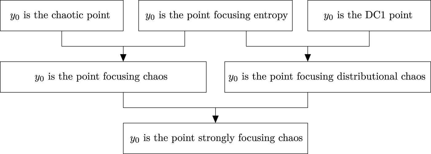
Many mathematicians connect various versions of chaos with positive entropy. For example, in [7], one can find the sentence “It is commonly accepted that an evidence of chaos is positivity of topological entropy.” Taking this into account, let us introduce the following definitions. We say that x 0 is a point focusing chaos if it is simultaneously a chaotic point and a point focusing entropy. We say that x 0 is a point focusing distributional chaos if it is simultaneously a DC1 point and a point focusing entropy. We say that x 0 is a point strongly focusing chaos if it is simultaneously a point focusing chaos and a point focusing distributional chaos. The relationship presented earlier is illustrated in the diagram.

Considerations connected with different kinds of chaos, also in the local aspects, require an examination of the interdependence of these concepts. We consider this problem in connection with the space of periodic non-autonomous dynamical systems.

In this way, we have defined the auxiliary dynamical system ( ξ 1 , ∞ ) , which will be used in proofs of all parts of this theorem.

To avoid repeating in respective parts of the proof, we will define some dynamical system ( g 1 , ∞ ) . For this purpose, we will consider a continuous function τ : [ 0 , 1 ] → [ 0 , 1 ] , which will satisfy the conditions (7). In the following parts of the proof, we will define functions τ a , τ b , τ c , and τ d (depending on demands of (a), (b), (c), and (d)) that meet the conditions (7). Then in each part, we will consider suitable dynamical systems ( g 1 , ∞ ) .

So, let T be a family of continuous functions τ : I → I , such that

First, we describe a finite sequence { g j } j = 1 k . If k = 1 , then the sequence { g j } j = 1 k consists of only one function, namely, g 1 = τ ∘ ξ 1 . In this case, ξ 1 ∣ [ y 0 − δ ∗ , y 0 + δ ∗ ] = id ∣ [ y 0 − δ ∗ , y 0 + δ ∗ ] , and hence, g 1 ∣ [ y 0 − δ ∗ , y 0 + δ ∗ ] = τ ∣ [ y 0 − δ ∗ , y 0 + δ ∗ ] . If k > 1 , then { g j } j = 1 k is a finite sequence of functions such that g j = ξ j for j ∈ 〚 1 , k − 1 〛 and g k = τ ∘ ξ k .

Notice useful properties of the sequence { g j } j = 1 k − 1 . From (5), we conclude

and hence,

Now we may consider the dynamical system ( g 1 , ∞ ) = ( g 1 , … , g k , g 1 , … , g k , … ) , having the period k . Obviously, g n k + 1 k = g 1 k and g 1 p k = g 1 ( p − 1 ) k ∘ g 1 k for n ∈ N 0 , p ∈ N + . Moreover, we have

Consequently,

Fix i ∈ N 0 . There exist p ∈ N 0 and q ∈ 〚 0 , k − 1 〛 such that i = p k + q . Then

Now fix s ∈ N 0 . There exist p ∈ N 0 and r ∈ 〚 0 , k − 1 〛 such that s = p k + r . Then g 1 k + s ( x ) = g 1 r ( τ p + 1 ( x ) ) for x ∈ [ y 0 − δ ∗ , y 0 + δ ∗ ] .

An easy verification shows that ρ ( g 1 , ∞ , ξ 1 , ∞ ) ≤ ε 2 . Hence, taking into account (6), we obtain ρ ( g 1 , ∞ , f 1 , ∞ ) < ε .

Observation. The reasoning carried out allows us to conclude that for any dynamical system ( g 1 , ∞ ) , constructed in the aforementioned way by means of functions fulfilling the conditions (7), the inequality ρ ( g 1 , ∞ , f 1 , ∞ ) ≤ ε takes place. Taking into account the arbitrariness of ε > 0 and the fact that ( f 1 , ∞ ) ∈ U I p , one can conclude that each family of dynamical systems constructed in this way is dense in U I p .

In order to simplify the construction of the “ τ function” for individual cases considered in this theorem, we will define the additional auxiliary function G : y 0 + δ ∗ 2 , y 0 + δ ∗ → R . For this purpose, we first consider

References

[1] L. Alsedá, J. Llibre, and M. Misiurewicz, Combinatorial Dynamics and Entropy in dimension One, second edition, Advanced Series in Nonlinear Dynamics, vol. 5. World Scientific Publishing Co. Inc., River Edge, NJ, 2000. 10.1142/4205Search in Google Scholar
[2] F. Balibrea and L. Rucká, Local distributional chaos, Qualitative Theory of Dynamical Systems 21 (2022), 130, DOI: https://doi.org/10.1007/s12346-022-00661-3. 10.1007/s12346-022-00661-3Search in Google Scholar
[3] L. S. Block and W. A. Coppel, Dynamics in one dimension, Lecture Notes in Mathematics, Springer, Berlin, 1992. 10.1007/BFb0084762Search in Google Scholar
[4] J. Dvořáková, Chaos in non-autonomous discrete dynamical systems, Commun. Nonlinear Sci. Numer. Simul. 17 (2012), 4649–4652. 10.1016/j.cnsns.2012.06.005Search in Google Scholar
[5] S. Kolyada and L. Snoha, Topological entropy of non-autonomous dynamical systems, Random Comput Dyn. 4 (1996), no. 2 & 3, 205–233. Search in Google Scholar
[6] E. Korczak-Kubiak and R. J. Pawlak, On local aspects of entropy, In: J. Awrejcewicz, (eds) Dynamical Systems in Theoretical Perspective, DSTA 2017. Springer Proceedings in Mathematics & Statistics, vol. 248, Springer, Cham, 2018, pp. 271–282. 10.1007/978-3-319-96598-7_22Search in Google Scholar
[7] D. Kwietniak and P. Oprocha, Topological entropy and chaos for maps induced on hyperspaces, Chaos Soliton Fractal. 33 (2007), 76–86. 10.1016/j.chaos.2005.12.033Search in Google Scholar
[8] T. Y. Li and J. Yorke, Period three implies chaos, Amer. Math. Month. 82 (1975), 985–992. 10.1080/00029890.1975.11994008Search in Google Scholar
[9] J. Li and X. Ye, Recent development of chaos theory in topological dynamics, Acta Math. Sin. English Ser. 32 (2016), 83–114. 10.1007/s10114-015-4574-0Search in Google Scholar
[10] A. Loranty and R. J. Pawlak, On the local aspects of distributional chaos, Chaos 29 (2019), Article ID 013104, p. 10. 10.1063/1.5046457Search in Google Scholar PubMed
[11] R. J. Pawlak, Distortion of dynamical systems in the context of focusing the chaos around the point, Int. J. Bifur. Chaos 28 (2018), no. 1, Article ID 1850006, p. 13. 10.1142/S0218127418500062Search in Google Scholar
[12] R. J. Pawlak and J. Poprawa, On generators and disturbances of dynamical system in the context of chaotic points, Bulletin Austr. Math. Soc. 100 (2019), no. 1, 1–10. 10.1017/S0004972718001454Search in Google Scholar
[13] S. Ruette, Chaos on the Interval, University Lecture Series, Vol. 67, American Mathematical Society, Providence, Rhode Island, 2017. 10.1090/ulect/067Search in Google Scholar
[14] B. Schweizer and J. Smítal, Measures of chaos and a spectral decomposition of dynamical systems on the interval, Trans. Am. Math. Soc. 344 (1994), 737–754. 10.1090/S0002-9947-1994-1227094-XSearch in Google Scholar
[15] X. Ye and G. Zhang, Entropy points and applications, Trans. Am. Math. Soc. 359 (2007), no. 12, 6167–6186. 10.1090/S0002-9947-07-04357-7Search in Google Scholar
Received: 2022-05-12
Revised: 2023-02-02
Accepted: 2023-02-13
Published Online: 2023-03-24
© 2023 the author(s), published by De Gruyter
This work is licensed under the Creative Commons Attribution 4.0 International License.
Articles in the same Issue
1. Research Articles
2. Asymptotic properties of critical points for subcritical Trudinger-Moser functional
3. The existence of positive solution for an elliptic problem with critical growth and logarithmic perturbation