Vanishing and blow-up solutions to a class of nonlinear complex differential equations near the singular point
-
Josef Diblík
 und
Miroslava Růžičková
und
Miroslava Růžičková

Abstract
A singular nonlinear differential equation
where
1 Introduction
A singular nonlinear differential equation
where
where
A proof is given of the existence of analytic solutions
Asymptotic analysis of equations in a neighbourhood of a singular point in the complex plane has a long history. In a pioneering article [3], a system of nonlinear differential equations and an initial problem
are considered with a function
and their modifications are investigated where
A substantial restriction used in the above-mentioned results is the assumption that
Moreover, the properties of solutions to systems (4) and (5) have only been studied in a subset of the origin (in a sector with its vertex at the point
In the right-hand side of (1), a “perturbation”
For the reader’s convenience, in Section 2, we recall some auxiliary notions and concepts well known from the theory of functions of complex variable. Transformations applied to equation (1) with focus on systems equivalent on given curves and rays to (1) are discussed in Section 3, while in Section 4, the behaviour of solutions is studied of the systems derived. In Section 5, the results of this article (Theorems 1–4) are formulated. Their proofs are given in Section 6. Since a major part of the proofs of Theorems 1–3 is identical for an arbitrary value of
2 Preliminaries
Consider an initial problem
where
Let
The concept of analytic continuation (extension) is used in this article as well. It means the following. Let
3 Transformations of equation (1)
Several auxiliary transformations of equation (1) are necessary for its analysis. In Section 3.1, we show why the coefficient
3.1 On the coefficient
a
in (1)
Let the complex coefficient
Then, a substitution, geometrically expressing a rotation,
where
with a positive coefficient
Therefore, the coefficient
3.2 Real system equivalent to (1) on the loops of a given curve
The behaviour of solutions to (1) in a small neighbourhood of the point
where
and, moreover, as we need
Inequality (9) will hold if and only if
and, obviously,
for
The closure of each loop of the curve (8) separated by an inequality (10) is a closed curve passing through the origin. If
Figure 1 shows different loops of (8) in the

Loops of (8) specified by
We will transform equation (1) into a system of two ordinary differential equations on parts of the closures of the loops of curve (8) with independent variable
where
Finally, using (8), (13), and (14),
Let
Equalling the real and imaginary parts, we see that
3.3 Real system equivalent to (1) on a system of rays
Consider rays running from the origin
and transform equation (1) along these into a system of two real equations. Since
(1) can be written as:
Assuming
Functions
4 Auxiliary results on the behaviour of solutions
In this section, we prove two lemmas used in proving the results of this article. In Section 4.1, the behaviour of solutions to (1) is considered along loop segments of the curve (8), while in Section 4.2, the behaviour of solutions to (1) is considered along rays (18) defined in Section 3.2.
4.1 Behaviour of solutions along segments of curve (8)
Assume, in the definition of curves (8),
In the following, we consider system (16), (17) in the domain
where
Let
where
Define cylinders
Lemma 1
Assume that
Then, any integral curve
behaves as follows. The integral curve
from domain
(26)into domain
(27)if
(28)holds for every admissible
Proof
Consider the behaviour of integral curves of system (16), (17) intersecting cylinders
we have
We will show that (29) implies
whenever (25) holds. Indeed, for
we have
Therefore, from (22), (23), and (25), it follows
Then, taking into account that
from (29), we derive
and (30) holds. Finally, we remark that (22), (23), and (25) imply
Remark 1
Note that the

Loops of (8) specified by
4.2 Behaviour of solutions along system of rays (18)
Assume, in the definition of rays (18),
i.e.
In this part, we will examine the behaviour of solutions to Systems (19) and (20) in the domain:
where
where
where
If an integral curve
where
by the definitions of
Lemma 2
Let
If
(36)Moreover,
(37)If
(38)and
(39)if
Proof
Let us investigate the behaviour of the integral curves intersecting cones
we have
where
Now, (40) will be used to determine
For
Then, by (33), (34), and (42),
and formula (41) holds. Therefore,
and
The geometric meaning of (43) is expressed by Inequality (36) in (i), which implies (37). Now, concerning conclusion (ii). In the case (44), we have
and this contradicts
Therefore, any solution
Remark 2
In this article, the existence of analytic solutions
if
5 Main results
This chapter is concerned with the existence of analytic solutions to (1) defined on subsets of neighbourhoods of the point
if the complex plane
if a Riemann surface
Define
and
Let
Before formulating Theorems 1–3, the following comments may be useful. Theorem 1 uses domains
while the second one by
provided that the parameter
respectively.
Theorem 2 uses domains
Similarly, domains
All the above-mentioned domains
For more details, we refer to Section 6. We refer as well to Figure 11 where the case
Theorem 1
Let
where
and inequality
Theorem 2
Let
where
and inequality
Theorem 3
Let
in a multiply-connected domain
where
and inequality
Remark 3
From the formulation of Theorem 1, it follows that the point
Theorem 4
Let
where
where
6 Proofs
The proofs are divided into several sections and are based on the results given in Sections 4.1 and 4.2. In Section 6.1, we show how the solution of an initial Cauchy problem to (1) can be analytically continued using given loops and rays in a domain
6.1 Analytic solutions on a domain
P
n
ω
In Section 6.1.1, we show how the solution of a Cauchy problem can be analytically continued using some of the previously defined curve loops and segments of rays, while in Section 6.1.3, using some properties of loop segments given in Section 6.1.2, this solution is analytically continued in a domain
6.1.1 Basic constructions using curve arcs and rays
Let, in (18),
where
and (31) holds. Let
be fixed, where
where
by the method of analytic continuation using the previously defined curves and rays. In Example 1, the following constructions are used as shown in Figure 3.

Visualization – to Example 1.
By Lemma 2, part (ii), with
preserves the property (54). We refer to Remark 2, where an explanation is given of the behaviour of solutions as
Consider segments of two loops of the curve (8), where either
and the angle
In (56), the number
for an arbitrary but fixed
Since the construction of
and
respectively. Assumption (21) is satisfied since
Therefore, for
so that
and
Assume that (63) holds. Then, both the above-mentioned segments intersect the ray (18), where
provided that (deducting from (55))
where
If the parameter
This maximum will be achieved for
or
From formulas (67) and (68) we deduce the following. If, for an increasing
with (63) still holding for all
Therefore, if
with
where
Let
holds for every
and
Along arcs (70), where
and, by Lemma 1, where
If domain (72) is considered, then, by (62),
and by part (ii) of Lemma 1, where
because
Moreover, by (50), (47), and (48), we have
Then, putting
the solution
for sufficiently small
Remark 4
The following property should be added to the previous consideration. Let
or
Since, in both cases,
for a sufficiently small
Example 1
Assume that, in equation (1), we have
Moreover, for
or
and, by (22), we can set (in the formula, the dependence on
In accordance with (56), define a range for
we can put, independently of
Now, consider a value
and we put
Then, by (65),
and the solution of equation (66)
gives the value
we can put (referring to (69))
Then,
The curve arcs (70) are defined by the angles
that are parts of domains (60) and (61), i.e.
respectively. Figure 3 shows the segments of the curve loops defined by (70), i.e.
passing through points
is analytically continued. Note that, for different values of
6.1.2 Auxiliary lemma
The following Lemma 3 and Remark 5 on the mutual positions of different segments of the loops of curve (8) will be used in further constructions. Instead of

Lemma 3
Let numbers
Consider two curve arcs
where
and
If
then
Proof
From (80)–(82), we see that (83) implies
Now, on the interval
By (85),
Due to (79), we have
and, analysing (87), we have
and
Due to (79), we have
and, consequently,
Therefore,
The general solution of (88) is
where, for the specification of arbitrary constants
The solution of the problem (88) is
The angle
For such values of
From this inequality, we deduce that
This inequality is equivalent with (84).□
Remark 5
A property similar to that formulated in Lemma 3, i.e. the inequality
can be proved in much the same way, if the following segments of loops are considered instead of (80) and (81):
Example 2
We use some constructions from Example 1 to illustrate Lemma 3 and Remark 5. We refer to Figure 4 where the two red and two green loop segments can be seen passing through the point
where
while the outer green one is defined by the formula:
where
The inner red segment is defined by the formula:
where
while the outer red one is defined by the formula:
where
Assumption (83) holds since
and
This is in accordance with the assertions of Lemma 3 and Remark 5.
Remark 6
Let us point out another property of the mutual position of different segments of loops of the curve (8), which is obvious. If two segments
and
where
The same property holds if

Example 3
In the following, some constructions from Example 1 are used to illustrate the assertions of Remark 6. We refer to Figure 5 where the two red and two green loop segments are visualized passing through the points
where
while the outer green one is defined by the formula:
where
The inner red loop segment is defined by the formula:
where
while the outer red one is defined by the formula:
where
We see that
and
This is in accordance with the assertions of Remark 6.
6.1.3 Continuation of
w
n
0
(
z
)
to a domain
P
n
ω
Let
From the method of construction and (56), (71), (72), and (73), it follows that the domain
The sector
Assume now that
If
If
If
The domain
and passing through the point
and passing through the point

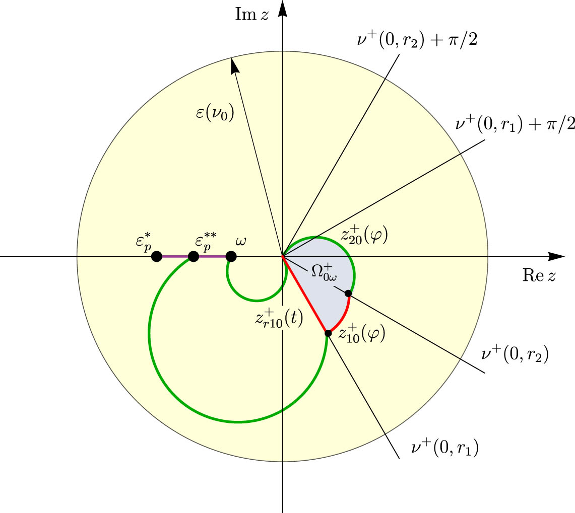
To Example 4 – domain
Example 4
Using several constructions of Example 1 again, we will construct the domain
where
while the green one in Figure 6, is defined as:
where
The outer boundary of
where
while the green one in Figure 6 is defined as:
where
6.2 Continuation of
w
n
0
(
z
)
from
P
n
ω
to domains
Ω
n
ω
+
and
Ω
n
ω
−
The solution
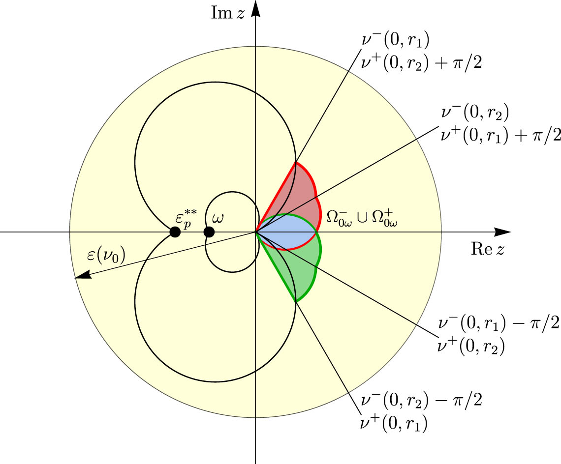
To Example 5 – domain

To Example 5 – domain
6.2.1 Construction of domain
Ω
n
ω
+
A domain
parts of the rays (18), where the angle
(97)and
Now, let us describe the construction in detail. We will generate the boundary of
where
Next, define the value
The first segment
where the parameter
The second segment
where the value of parameter
The segment
is a part of the boundary as well. By construction,
for each
for each
Here are some properties of segments of the loops of curve (8) with
The second one, provided that
Without loss of generality, we can assume that
The analytic continuation along segments of the loop or ray has the following properties. Since
part (i) of Lemma 1 is applicable. Therefore, on the given loop segments,
For
Then, part (i) of Lemma 2 is applicable. Note that the value
is nonzero for every fixed
Thus, in Lemma 2, irrespective of the value
By (37), on a given ray
where
6.2.2 Construction of domain
Ω
n
ω
‒
Similarly, the domain
parts of the rays (106), where the angle
(113)and
The following computations is much the same as those in Section 6.2.1. We omit the details defining the boundary of
where
where
is part of the boundary as well. By construction,
where
where
The following are the properties of segments of loops of the curve (8) with
The second one, provided that
part (ii) of Lemma 1 is applicable. Therefore, on the given arcs,
part (i) of Lemma 2 is applicable. In Lemma 2, we can use, irrespectively of the value
where
6.2.3 Behaviour of
w
n
0
(
z
)
on domains
Ω
n
ω
+
and
Ω
n
ω
‒
From the constructions of domains
By Formulas (110) and (118), the convergence to zero has an exponential character.
Example 5
Let
where
The first loop segment
where
The parameter
and
and
where
Finally, by equation (106), the segment of the ray
The domain
where
By (115) and (116), for
where
Finally, by equation (117), the segment of the ray
The domain
To Example 5 – domain
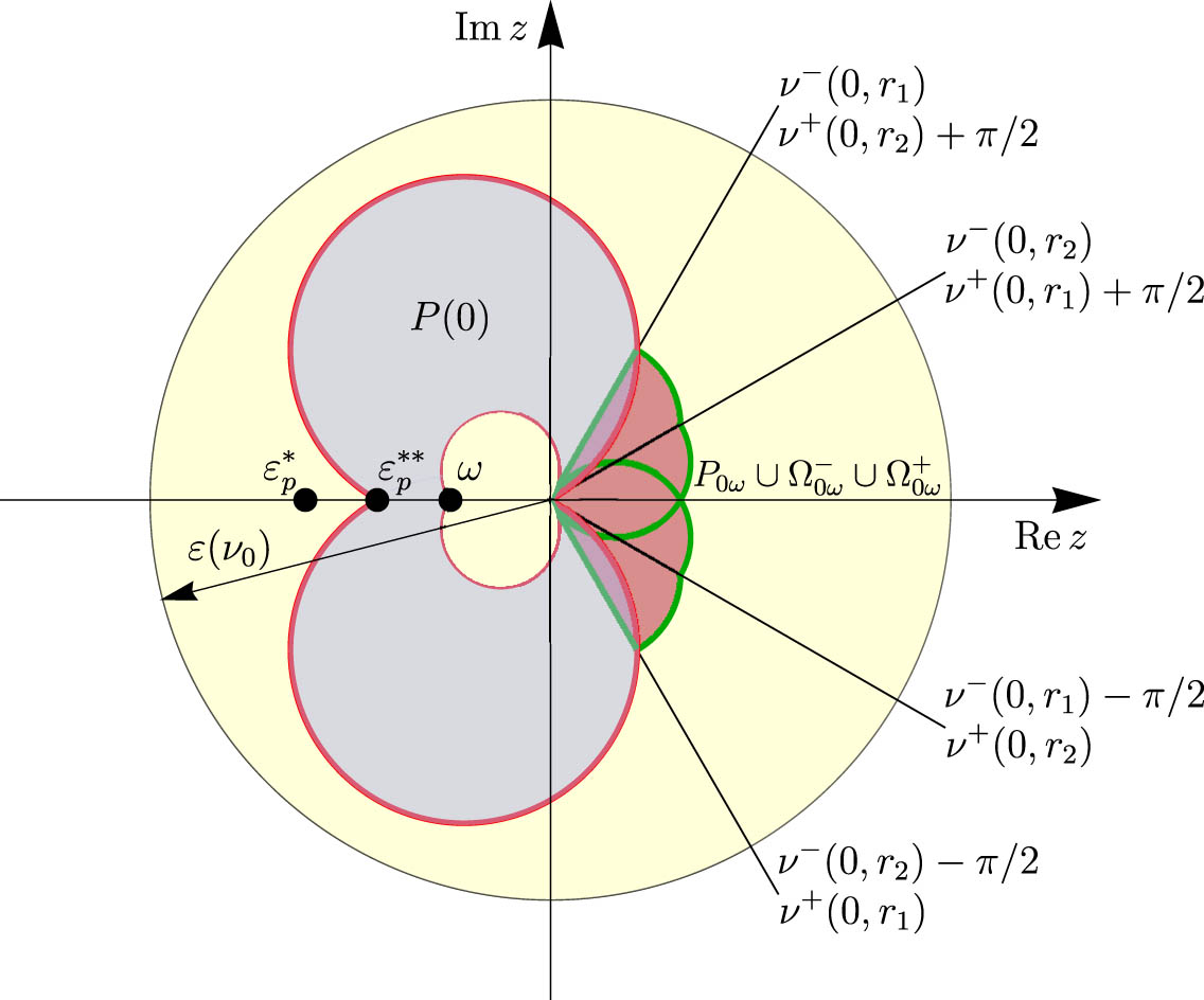
6.3 Domain
P
(
n
)
and property
P
(
n
)
∩
P
(
n
+
1
)
≠
∅
From the previous considerations, we conclude that the solution
Provided that
The last property follows from (47), (48), (56), (96), and (112) because, in the opposite case, the inequality
must hold. Simplifying (122), we obtain
Remark 7
In the following, we refer to Example 5. The domain
Inequality (49) is now
where

We will show that the intersection
This is a consequence of the fact that the angle
holds being equivalent with
Moreover, let
where
since the inequality
is equivalent to
6.4 Solutions analytically continuable to
P
(
n
)
∪
P
(
n
+
1
)
The following explanation can be followed in Figures 12 and 13, Example 5, and Remark 8. Let
where
Assume as well that, on the curve
while on the curve
To define the curve
and to define the curve
in (8). Then, the point of intersection
In the case of
The symmetry property can be proved in much the same way. The equations defining the curves
and
where


Remark 8
We use Example 5 again to visualize curves
and
where
Assuming that
where
Initially, we will examine the case of the curve
remains inside the cylinder if
being defined as its mapping by the corresponding integral curve when
This inequality holds, we refer to (125), (128), and also to Remark 1. The aforementioned mapping is continuous implementing a one-to-one correspondence between the lower base, i.e. the set
and a simply connected nonempty domain
In addition, to each point of the domain
On
remains inside the cylinder if
as a result of mapping along the corresponding integral curve when
In this case, the upper base of cylinder (131), i.e. the set
is mapped into a simply connected nonempty domain
By construction, to each point of the domain
Neither of the domains
since the system (16), (17) has a trivial solution
Thus, the set
6.5 Solutions analytically continuable to
P
(
n
)
∪
P
(
n
+
1
)
∪
P
(
n
+
2
)
Let us repeat the considerations of the previous section for the domain:
Now, adapting the previous notation, the set
Then, there exists a compact two-dimensional set
6.6 Solutions analytically continuable to
P
(
n
)
∪
⋯
∪
P
(
n
+
N
)
Let the above-mentioned construction be carried out for each fixed integer
If
where
If
where
If
located on the Riemann surface of the logarithmic function.
7 Example
Let, in an equation (1),
and there are two different values for
Next, we apply formula (34) with
Let
and the solution of equation (66)
gives the value
By (22), we can put
we can, independently of
we can put
For completeness, we compute the angles, defined by (47) and (48):
Now, let us construct the domains
where
while the green one is defined as:
where
The outer boundary of
where
while the green one is defined as:
where
The inner boundary of
where
while the green one is defined as:
where
The outer boundary of
where
while the green one is defined as:
where
Figure 15 shows a circle neighbourhood of the origin in
The curve
where the value of the parameter
and
The curve
where the value of parameter
and
Then,
Since
where

Case
Case
8 Concluding remarks and open problems
Part 5 gives a detailed description of simply connected domains (blow-up holes) of the type
and, in the constructions, the positive number
Being geometrical, the method used is suitable for analysing the behaviour of solutions near singular points. When investigating equation (1), two singular systems are considered of ordinary differential equations. The first one is derived as a system along the curves defined by Formula (8), the second one is a system corresponding to rays (18) originating at point
Acknowledgements
Both authors studied in the seventies at Odessa I. I. Mechnikov National University under the supervision of Professor R. G. Grabovskaya. We are much indebted to her for supervising us in the field of applicability of geometrical methods in qualitative analysis of differential equations leading, in particular, to results presented in this study. This article is dedicated to her memory.
-
Funding information: Josef Diblík has been supported by the projects of specific university research FAST-S-22-7867 (Faculty of Civil Engineering, Brno University of Technology) and FEKT-S-23-8179 (Faculty of Electrical Engineering and Communication, Brno University of Technology). The research of Miroslava Růžičková was supported by the Polish Ministry of Science and Higher Education under a subsidy for maintaining the research potential of the Faculty of Mathematics, University of Białystok, Poland.
-
Conflict of interest: The authors state no conflict of interest.
References
[1] J. A. D. Appleby and D. D. Patterson, Growth and fluctuation in perturbed nonlinear Volterra equations, Appl. Math. Comput. 396 (2021), Paper No.125938, 1–34. 10.1016/j.amc.2020.125938Suche in Google Scholar
[2] J. A. D. Appleby and D. D. Patterson, Growth rates of solutions of superlinear ordinary differential equations, Appl. Math. Lett. 71 (2017), 30–37. 10.1016/j.aml.2017.03.012Suche in Google Scholar
[3] C. A. A. Briot and J. C. Bouquet, Recherches sur les propriétés des fonctions définies par des équations différentielles, J. École Polytechnique 36 (1856), 133–198. Suche in Google Scholar
[4] S. Cherief and S. Hamouda, Growth of solutions of a class of linear differential equations near a singular point, Kragujevac J. Math. 47 (2023), no. 2, 187–201. 10.46793/KgJMat2302.187CSuche in Google Scholar
[5] J. Diblík and Chr. Nowak, A nonuniqueness criterion for a singular system of two ordinary differential equations, Nonlinear Anal. 64 (2006), no. 4, 637–656. 10.1016/j.na.2005.05.042Suche in Google Scholar
[6] J. Diblík and M. Růžičková, Inequalities for solutions of singular initial problems for Carathéodory systems via Ważewski’s principle, Nonlinear Anal. 69 (2008), no. 12, 4482–4495. 10.1016/j.na.2007.11.006Suche in Google Scholar
[7] A. Domoshnitsky, Nonlinear problems with blow-up solutions: numerical integration based on differential and nonlocal Unboundedness of solutions and instability of differential equations of the second order with delayed argument, Differential Integral Equations 14 (2001), no. 5, 559–576. 10.57262/die/1356123256Suche in Google Scholar
[8] V. V. Golubev, Lekcii po analitičeskoĭ teorii differencial’nyh uravnenĭ (Russian), Lectures on the Analytic Theory of Differential Equations, 2nd ed., Gosudarstv. Izdat. Tehn.-Teor. Lit., Moscow-Leningrad, 1950. Suche in Google Scholar
[9] R. G. Grabovskaya, The asymptotic behavior of the solutions of a certain system of first order nonlinear differential equations, Dopovidi Akad. Nauk Ukrain. RSR Ser. A 1969 (1969), 867–871, (Ukrainian). Suche in Google Scholar
[10] R. G. Grabovskaya, The asymptotic behavior of the solution of a system of two first order nonlinear differential equations, Differencial’nye Uravnenija 11 (1975), no. 4, 639–644, (Russian). Suche in Google Scholar
[11] I. Györi, Y. Nakata, and G. Röst, Unbounded and blow-up solutions for a delay logistic equation with positive feedback, Commun. Pure Appl. Anal. 17 (2018), no. 6, 2845–2854. 10.3934/cpaa.2018134Suche in Google Scholar
[12] S. Hamouda, The possible orders of growth of solutions to certain linear differential equations near a singular point, J. Math. Anal. Appl. 458 (2018), no. 2, 992–1008. 10.1016/j.jmaa.2017.10.005Suche in Google Scholar
[13] M. Hukuhara, Intégration formelle d’un système d’équations of différentielles non-linéaris dans le voisinage d’un point singulier, Ann. Math Pura Appl. Bologna 19 (1940), no. 4, 35–44. 10.1007/BF02410538Suche in Google Scholar
[14] M. Hukuhara, La direction de Julia au point singulier fixe d’une équation différentielle ordinaire du premier ordre, Japanese J. Math. 29 (1960), 5–8. 10.4099/jjm1924.29.0_5Suche in Google Scholar
[15] P.-F. Hsieh and Y. Sibuya, Basic Theory of Ordinary Differential Equations, Universitext, Springer-Verlag, New York, 1999. 10.1007/978-1-4612-1506-6Suche in Google Scholar
[16] P.-F. Hsieh, On a reduction of nonlinear ordinary differential equations at an irregular type singularity, Arch. Math. (Brno) 10 (1974), no. 3, 129–147. Suche in Google Scholar
[17] P.-F. Hsieh, Recent advances in the analytic theory of nonlinear differential equations with an irregular type singularity, International Conference on Differential Equations, University of Southern California, on September 3–7, 1974, pp. 370–384, Edited by H. A. Antosiewicz, Academic Press, University of Southern California, 1975, 856 pp. 10.1016/B978-0-12-059650-8.50034-XSuche in Google Scholar
[18] T. Ishiwata and Y. Nakata, A note on blow-up solutions for a scalar differential equation with a discrete delay, Jpn. J. Ind. Appl. Math. 39 (2022), no. 3, 959–971. 10.1007/s13160-022-00533-ySuche in Google Scholar
[19] M. Ivano, Analytic expressions for bounded solutions of nonlinear ordinary differential equations with on irregular type singular point, Ann. Math. Pure Appl. 82 (1969), 182–256. 10.1007/BF02410798Suche in Google Scholar
[20] M. Ivano, Bounded solutions and stable domains of nonlinear ordinary differential equations, Analytic Theory of Differential Equations (Proc. Conf., Western Michigan Univ., Kalamazoo, Mich., 1970), Lecture Notes in Mathematics, Vol. 183, Springer, Berlin, 1971, pp. 59–127, Lecture Notes in Math., Vol. 183, Springer, Berlin, 1971. 10.1007/BFb0060412Suche in Google Scholar
[21] M. Ivano, Intégration analytique d’un système d’équations of différentielles non-linéaris dans le voisinage d’un point singulier I, Appl. Math. Comput. 4 (1959), no. 44, 261–292. 10.1007/BF02415204Suche in Google Scholar
[22] M. Ivano, Intégration analytique d’un système d’équations of différentielles non-linéaris dans le voisinage d’un point singulier II, Appl. Math. Comput. 4 (1959), no. 47, 91–149. 10.1007/BF02410894Suche in Google Scholar
[23] M. Ivano, On a general solution of a nonlinear n -system of the form x2dy∕dx=(1n(μ)+x1n(α))y+xf(x,y) with a constant diagonal matrix 1n(μ) of signature (m,n−m), Ann. Mat. Pura Appl. 130 (1982), no. 4, 331–384. 10.1007/BF01761502Suche in Google Scholar
[24] M. Kirane, A. Alsaedi, and B. Ahmad, Blowing-up solutions of differential equations with shifts: A survey, Discrete Contin. Dyn. Syst. Ser. S 16 (2023), 1537–1556. 10.3934/dcdss.2022100Suche in Google Scholar
[25] D. E. Limanska, On the behavior of the solutions of some systems of differential equations partially solved with respect to the derivatives in the case with a pole, Nelïnïǐnï Koliv. 20 (2017), no. 1, 113–126, (Russian), translation in J. Math. Sci. (N.Y.)229 (2018), no. 4, 455–469. 10.1007/s10958-018-3689-0Suche in Google Scholar
[26] D. E. Limanska and G. E. Samkova, On the existence of analytic solutions of certain types of systems, partially resolved relatively to the derivatives in the case of a pole, Mem. Differ. Equ. Math. Phys. 74 (2018), 113–124. Suche in Google Scholar
[27] J. Malmquist, Sur les points singuliers des équations différentielles, Ark. Mat. Astr. Fys. 29A (1943), no. 18, 1–11. Suche in Google Scholar
[28] A. Polyanin and I. K. Shingareva, Non-monotonic blow-up problems: test problems with solutions in elementary functions, numerical integration based on non-local transformations, Appl. Math. Lett. 76 (2018), 123–129. 10.1016/j.aml.2017.08.009Suche in Google Scholar
[29] A. Polyanin and I. K. Shingareva, Nonlinear problems with blow-up solutions: numerical integration based on differential and nonlocal transformations, and differential constraints, Appl. Math. Comput. 336 (2018), 107–137. 10.1016/j.amc.2018.04.071Suche in Google Scholar
[30] W. Wasow, Asymptotic Expansions for Ordinary Differential Equations, Dover Publications, United States, 2018. Suche in Google Scholar
[31] D. Westreich and E. Podolak, Systems of Briot-Bouquet equations with analytic solutions, Canad. Math. Bull. 25 (1982), no. 2, 230–233. 10.4153/CMB-1982-032-0Suche in Google Scholar
© 2024 the author(s), published by De Gruyter
This work is licensed under the Creative Commons Attribution 4.0 International License.
Artikel in diesem Heft
- Regular Articles
- Existence of normalized peak solutions for a coupled nonlinear Schrödinger system
- Orbital stability of the trains of peaked solitary waves for the modified Camassa-Holm-Novikov equation
- Global boundedness in a two-dimensional chemotaxis system with nonlinear diffusion and singular sensitivity
- Existence and uniqueness of solution for a singular elliptic differential equation
- The bounded variation capacity and Sobolev-type inequalities on Dirichlet spaces
- Vanishing and blow-up solutions to a class of nonlinear complex differential equations near the singular point
- Existence, uniqueness, localization and minimization property of positive solutions for non-local problems involving discontinuous Kirchhoff functions
- Concentration phenomena for a fractional relativistic Schrödinger equation with critical growth
- Beyond the classical strong maximum principle: Sign-changing forcing term and flat solutions
- Monotonicity of solutions for parabolic equations involving nonlocal Monge-Ampère operator
- On a nonlinear Robin problem with an absorption term on the boundary and L1 data
- Multiple solutions for the quasilinear Choquard equation with Berestycki-Lions-type nonlinearities
- Gradient estimates for a class of higher-order elliptic equations of p-growth over a nonsmooth domain
- Global existence and decay estimates of the classical solution to the compressible Navier-Stokes-Smoluchowski equations in ℝ3
- Global existence and finite-time blowup for a mixed pseudo-parabolic r(x)-Laplacian equation
- Multiple positive solutions for a class of concave-convex Schrödinger-Poisson-Slater equations with critical exponent
- A minimization problem with free boundary for p-Laplacian weakly coupled system
- Multiplicity of semiclassical solutions for a class of nonlinear Hamiltonian elliptic system
- k-convex solutions for multiparameter Dirichlet systems with k-Hessian operator and Lane-Emden type nonlinearities
- Infinitely many solutions for Hamiltonian system with critical growth
- On optimal control in a nonlinear interface problem described by hemivariational inequalities
- Variational–hemivariational system for contaminant convection–reaction–diffusion model of recovered fracturing fluid
- Potential and monotone homeomorphisms in Banach spaces
- Critical fractional Schrödinger-Poisson systems with lower perturbations: the existence and concentration behavior of ground state solutions
- Supercritical Hénon-type equation with a forcing term
- Concentration of blow-up solutions for the Gross-Pitaveskii equation
- Mountain-pass-type solutions for Schrödinger equations in R2 with unbounded or vanishing potentials and critical exponential growth nonlinearities
- Regularity for critical fractional Choquard equation with singular potential and its applications
- Double phase anisotropic variational problems involving critical growth
- Normalized solutions of NLS equations with mixed nonlocal nonlinearities
- Nontrivial solutions for resonance quasilinear elliptic systems
- Standing waves for Choquard equation with noncritical rotation
- Low regularity conservation laws for Fokas-Lenells equation and Camassa-Holm equation
- Modified quasilinear equations with strongly singular and critical exponential nonlinearity
- Limit profiles and the existence of bound-states in exterior domains for fractional Choquard equations with critical exponent
- Nests of limit cycles in quadratic systems
- Regularity of minimizers for double phase functionals of borderline case with variable exponents
- Boundedness, existence and uniqueness results for coupled gradient dependent elliptic systems with nonlinear boundary condition
- Ground state solutions for magnetic Schrödinger equations with polynomial growth
- Nonoccurrence of Lavrentiev gap for a class of functionals with nonstandard growth
- Dynamics for wave equations connected in parallel with nonlinear localized damping
- Boussinesq's equation for water waves: Asymptotics in Sector I
- Optimal global second-order regularity and improved integrability for parabolic equations with variable growth
- Normalized solutions of Schrödinger equations involving Moser-Trudinger critical growth
- Normalized solutions for the double-phase problem with nonlocal reaction
- Normalized solutions for Sobolev critical fractional Schrödinger equation
- Well-posedness of Cauchy problem of fractional drift diffusion system in non-critical spaces with power-law nonlinearity
- Improved results on planar Klein-Gordon-Maxwell system with critical exponential growth
- Existence and multiplicity of solutions for a new p(x)-Kirchhoff equation
- Quasiconvex bulk and surface energies: C1,α regularity
- Time decay estimates of solutions to a two-phase flow model in the whole space
- Bounds for the sum of the first k-eigenvalues of Dirichlet problem with logarithmic order of Klein-Gordon operators
- The properties of a new fractional g-Laplacian Monge-Ampère operator and its applications
- A fractional profile decomposition and its application to Kirchhoff-type fractional problems with prescribed mass
- Cauchy problem for a non-Newtonian filtration equation with slowly decaying volumetric moisture content
- Multiplicity of normalized semi-classical states for a class of nonlinear Choquard equations
- The second Yamabe invariant with boundary
- Peaked solitary waves and shock waves of the Degasperis-Procesi-Kadomtsev-Petviashvili equation
- Normalized solutions for the Choquard equations with critical nonlinearities
- Boundedness and long-time behavior in a parabolic-elliptic system arising from biological transport networks
- Initial boundary value problem and exponential stability for the planar magnetohydrodynamics equations with temperature-dependent viscosity
- Nonexistence of mean curvature flow solitons with polynomial volume growth immersed in certain semi-Riemannian warped products
- Analysis of a vector-borne disease model with vector-bias mechanism in advective heterogeneous environment
- Normalized solutions for the Kirchhoff equation with combined nonlinearities in ℝ4
- Nonexistence of the compressible Euler equations with space-dependent damping in high dimensions
- Multiplicity of solutions for a nonhomogeneous quasilinear elliptic equation with concave-convex nonlinearities
- On semilinear inequalities involving the Dunkl Laplacian and an inverse-square potential outside a ball
- Besov regularity for the elliptic p-harmonic equations in the non-quadratic case
-
Uniqueness and nondegeneracy of ground states for
- Existence of solutions for a class of quasilinear Schrödinger equations with Choquard-type nonlinearity
- Weighted Hardy-Adams inequality on unit ball of any even dimension
- Existence and regularity for a p-Laplacian problem in ℝN with singular, convective, and critical reaction
- Temporal periodic solutions of non-isentropic compressible Euler equations with geometric effects
- Nodal solutions for a zero-mass Chern-Simons-Schrödinger equation
- The modified quasi-boundary-value method for an ill-posed generalized elliptic problem
- Nonlocal heat equations with generalized fractional Laplacian
- Choquard equations with recurrent potentials
- Local and global well-posedness of the Maxwell-Bloch system of equations with inhomogeneous broadening
- The Riemann problem for two-layer shallow water equations with bottom topography
- Global stability and asymptotic profiles of a partially degenerate reaction diffusion Cholera model with asymptomatic individuals
- On Kirchhoff-Schrödinger-Poisson-type systems with singular and critical nonlinearity
- Energy-variational solutions for viscoelastic fluid models
- Stability on 3D Boussinesq system with mixed partial dissipation
- Existence and multiplicity results for non-autonomous second-order Hamiltonian systems
- Erratum
- Erratum to “Normalized solutions for the Kirchhoff equation with combined nonlinearities in ℝ4”