
Geometry of the Rabi Problem and Duality of Loops
-
Heinz-Jürgen Schmidt


Abstract
We investigate the motion of a classical spin processing around a periodic magnetic field using Floquet theory, as well as elementary differential geometry and considering a couple of examples. Under certain conditions, the role of spin and magnetic field can be interchanged, leading to the notion of “duality of loops” on the Bloch sphere.
1 Introduction
The Rabi problem usually refers to the response of an atom to an applied harmonic electric field, with an applied frequency very close to the atom’s natural frequency [1], [2]. Assuming that the atom can be approximated by a two-level system, its semiclassical Hamiltonian (in the sense that the radiation field is treated classically) will be of the form of a Zeeman term in an s = 1/2 spin system:
where the Sx, Sy, Sz are the s = 1/2 spin operators. If ψ(t) is a solution of the corresponding Schrödinger equation (ℏ = 1):
then the projector
It follows that
as a classical magnetic moment performing a Larmor precession around the time-dependent periodic magnetic field
To illustrate the preceding remarks, consider the textbook example of the circularly polarised Rabi problem with
A special solution of the corresponding Schrödinger equation (2) is the following:
where Δ is the “detuning”
and Ω denotes the “Rabi frequency”
This solution demonstrates the well-known Rabi oscillations of the occupation numbers of the eigenstates of the static Hamiltonian according to
However, the projector
On the other hand, it can be shown [5], [6] that in the general case of periodic
We mention in passing that solutions of the classical Rabi problem also yield solutions of the quantum Rabi problem for arbitrary spin quantum number s. This follows either from representation theory [5] or by using the Majorana stellar representation [8] of spin states by
The differential equation (4) can be explicitly solved only in a few cases of physical interest. The most prominent one, already mentioned above, is a constant field superimposed by a monochromatical, circularly polarised field perpendicular to the constant one [1]. The analogous problem with a linearly polarised field component is solvable in terms of confluent Heun functions [10], [11], [12], [13] for the corresponding s = 1/2 Schrödinger equation. In this article, we will shift the problem of finding solutions of (2) or (4) to the study of geometric relations between such solutions and to the interplay between Floquet theory, differential geometry of the unit sphere, and duality of loops. Not all results will be new, but we will provide new proofs that only use properties of solutions of the classical Rabi problem that are easier to visualise and do not resort to the mathematics of the underlying Schrödinger equation. Obviously, there exist close connections between the present article and the theory of geometric phases, initiated by M. Berry [14], generalised by [15], and still a topic of current experimental research (e.g. [16], [17], [18], [19]). However, a detailed account of these connections cannot be given here and must be left for future publications.
2 Periodic Solutions
We will sketch the essential arguments leading to periodic solutions of the classical Rabi problem and the reconstruction of the (time-depending) phase factor. First, we may apply the Floquet theory [20], [21] to the Schrödinger equation (2) and conclude that it has special solutions (“Floquet solutions”) of the form
such that
and these will be chosen in the sequel. It follows immediately that the projectors
Conversely, let a T-periodic solution of (4) be given and
It follows that
and hence
where (16) represents the Fourier series of the T-periodic function (15). The integration of (16) yields
and hence, ψ(t) will be a Floquet solution of the form
with quasienergy
It will be instructive to consider another argument leading to a periodic solution of (4). To this end, we consider a
the latter denoting the
where
and the
represents the axis of rotation and, after normalisation
and hence,
The angle of rotation δ ≥ 0 corresponding to
This follows from [5] by the “lift” from s = 1/2 to s = 1. Independently, one may directly prove the proposition by considering the unitary matrix of Floquet solutions
and the superposition
Here
and
are T-periodic functions satisfying
for all
and
Hence,
as can be shown by a straightforward calculation. This completes the proof of Proposition 1. ⊡
In view of Proposition 1, we will define the “classical quasienergy” by
3 Quasienergy
It has been shown [5] that the quasienergy of the s = 1/2 Schrödinger equation (2) with a periodic magnetic field can be expressed in terms of integrals using the periodic solution of the analogous classical Rabi problem. Here we will rederive this result without employing the reference to the Schrödinger equation, solely by using the periodic solution
To this end, we consider a time-dependent right-handed orthonormal frame, shortly called “e frame,” defined by
Further, let
be a solution of (20) with initial conditions
and hence
for all
where
This result slightly improves the corresponding equation (62) in [5] in so far as it is manifestly independent of a coordinate system. The explicit accordance with [5] has been shown in [6]. We note that the form of (46) suggests the following splitting of the quasienergy:
into a “dynamical part”
For the geometrical part
where we have denoted the s derivative by a prime ′. This transformation produces a factor
Furthermore, for the calculation of
The following choices considerably simplify the calculations: As a parameter of 𝒮, we will use the arc length that will always be denoted by s in what follows. Differentiation with respect to s will again be denoted by a prime ′ without danger of confusion. The length of the curve 𝒮 will be denoted by
Further, we will choose as a suitable magnetic field
which will always be of unit length,
as the vector product of two orthogonal unit vectors. Equation (48) yields the correct spin curve 𝒮 as it satisfies
As
It is known from elementary differential geometry that the “geodesic curvature” kg of a curve 𝒮 on a surface parametrised by its arc length is defined as the triple product
measuring the component of the acceleration
Here M denotes a two-dimensional submanifold of S2 with boundary
The last term −2π is irrelevant as the quasienergy is only defined modulo
that endows
4 Duality of Loops
We start with a loop 𝒮 and its dual loop ℋ on the unit Bloch sphere parametrised by the arc length s of 𝒮 such that
and
(We will avoid the use of primes for derivatives in this section in order to avoid misunderstandings.) Hence, the triple
is orthogonal to h and s and hence must be proportional to
where
and hence
Now (58), (61), and (63) imply
The latter equation has the form of (4) and hence can be interpreted in such a way that the “spin vector” h moves according to (4) under the influence of the “magnetic field”
The situation will be more symmetric if we additionally pass from s to the arc length parameter of ℋ, denoted by r. Then, the equation of motion for
Now the new “magnetic field”
This means that
and hence
Together with (65), this implies
If the role of 𝒮 and ℋ is interchanged, we obtain
where G is the geodesic curvature of ℋ:
Using (59) and (63), we may rewrite (62) as
Then, it follows that
and hence
This means that, up to a possible sign, the geodesic curvature differential g ds of 𝒮 equals the arc length differential dr of ℋ. If g does not change its sign, both differentials can be integrated and yield identical integrals, up to a possible sign.
The curve 𝒮 will be called simple if its geodesic curvature does not change its sign. In this case, we obtain
and, by means of (56) and (57),
The result (75) reminds of the relationship between the geometric phase and the contracted length of the system’s path in projective Hilbert space according to [25].
Summarising, we have two loops 𝒮 and ℋ on the unit Bloch sphere that give rise to two different solutions of (4): Either 𝒮 consists of spin vectors or ℋ consists of magnetic field vectors, and the time parameter t in (4) is chosen as the arc length s of 𝒮. Or, ℋ consists of spin vectors and
For both realisations of solutions of (4), we can calculate the classical quasienergy denoted by
further illustrating the duality between 𝒮 and ℋ.
We note that there is still a minor asymmetry between the curves 𝒮 and ℋ of a dual pair, insofar the two branches
Still another way of looking at the duality of loops considered in this section would be based on the observation that the equation of motion (4) can be viewed as a Hamiltonian equation with a two-dimensional phase space S2 and the time-dependent Hamiltonian
see [5]. In the special case where t is the arc length parameter of 𝒮, it follows that
4.1 Example 1
In order to illustrate the notion of duality considered in this section, we consider two examples. The first one is a special case of the Rabi problem with circular polarisation. Let
be the arc length parametrisation of a circle 𝒮 on S2 lying in the plane z = const. with
Then, (59) yields the parametrisation of the dual loop ℋ:
satisfying
After some elementary calculations, we obtain
and hence, the first expression for the classical quasienergy
The solid angle enclosed by 𝒮 will be
and hence, a second expression for
It satisfies
and hence, both expressions (84) and (86) agree modulo ω.
The arc length parameter r corresponding to ℋ is obtained as
After some elementary calculations, we obtain
and hence, the first expression for the quasienergy
The solid angle enclosed by ℋ will be
and hence, a second expression for
It satisfies
the ± sign depending on the sign of z. Hence, both expressions (90) and (93) agree up to a sign and modulo Ω.
Equation (77) holds for the present example as the triple products g and G are constant and, due to (89), inverses of each other.
In the case of
see, e.g. [26]. In this sense, our definition of dual curves is compatible with the established notion of dual cones in ℝ3.
Finally, we note that the magnetic field (81) can be understood as a special case of the Rabi problem with circularly polarised driving (23), if we set
see [5], (8) and taking into account that the quasienergy of the classical Rabi problem is twice the quasienergy of the s = 1/2 quantum Rabi problem modulo ω, see also Proposition 1. In our case, it follows that
which agrees with (84) up to a possible sign.
4.2 Example 2
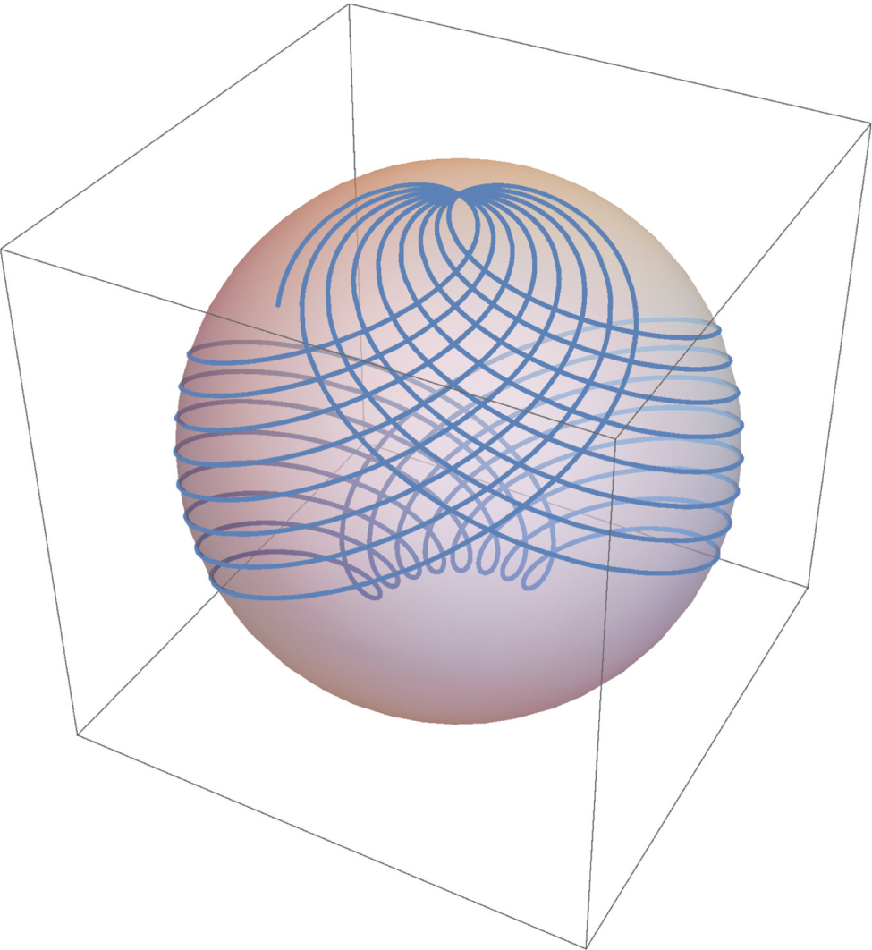
For the second example, we take a case where 𝒮 is not simple, but of the form of the figure “8” (lemniscate) with a self-intersection that is simultaneously a point of inflection. This example also shows that we need not explicitly calculate the arc length parameters s of 𝒮 or r of ℋ but may work within the initial parametrisation. Let the figure “8” curve be given by the parametrisation
where
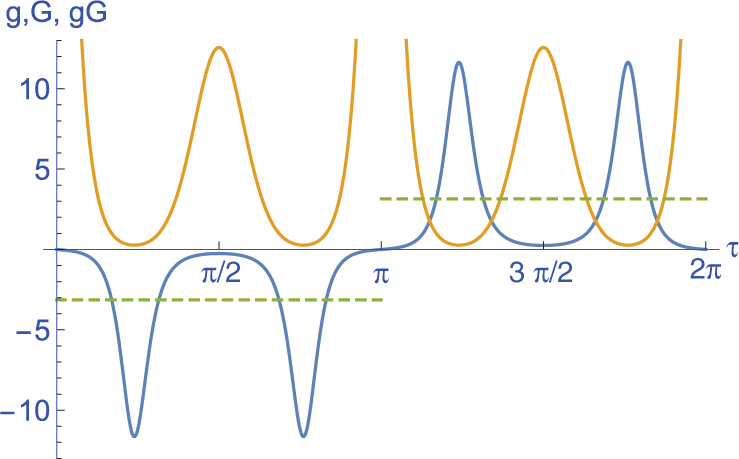
analogously to (59) but without directly using the arc length parameter s. This and the following expressions can be easily obtained by a computer algebra software but are too involved to be displayed here. The loop ℋ is displayed in Figure 2. It shows two cusps corresponding to the point of self-intersection of 𝒮. These cusps necessarily occur according to the following reasoning: At the point of self-intersection corresponding to the values τ = 0, π of the parameter, the geodesic curvature g of 𝒮 changes its sign (Fig. 3). According to (69), the geodesic curvature G of ℋ must diverge at τ = 0, π, which explains the two cusps.
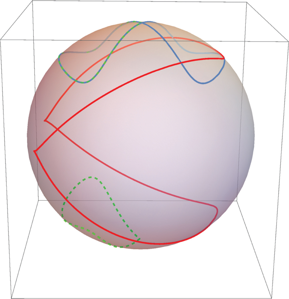
Illustration of example 2 for duality of loops. The blue (grey) curve represents the orbit 𝒮 of a time-dependent spin function
The curve 𝒮 can be divided into the parts 𝒮1 and 𝒮2 that have in common only the point of self-intersection. The corresponding parts of ℋ are denoted by
Interestingly, if we calculate the “bidual” loop ℛ according to
then, we obtain two disjoint curves that locally coincide with
5 Summary and Outlook
We have considered some geometrical aspects of the classical Rabi problem with arbitrary periodic driving. The classical equation of motion can be viewed in its own right as a case where Floquet theory can be applied, without resort to the underlying Schrödinger equation. In contrast to the latter, it has always some periodic solutions. This leads to the definition of the classical quasienergy
It is not straightforward to assess the possible benefits of the present results for concrete physical problems, also because of the diversity of such problems. However, as a rule, the solutions of the equations of motion of the classical spin can be more directly visualised than the solutions of the corresponding Schrödinger equation. Although this advantage is lost in higher-dimensional Hilbert spaces, it would be instructive to investigate which geometric properties remain invariant if we pass from the Bloch sphere to a higher-dimensional projective Hilbert space. The latter is known to be a Kähler manifold that carries two related structures, a Riemannian and a symplectic one, which can be used to obtain geometric phases in different ways [27], [28].
Acknowledgement
I thank the members of the DFG Research Unit FOR 2692 for stimulating and insightful discussions on the topic of this article. I am also grateful for valuable suggestions from some anonymous referees and their references to relevant literature.
Appendix A: Proof of the Integral Representation of the Classical Quasienergy
We use the abbreviation
and expand the magnetic field with respect to the e frame, defined in (38–40):
The equation
immediately implies
and moreover,
We will also expand
Second,
where we have abbreviated the triple product
With this, we can evaluate the t derivatives of the e frame vectors in the following way:
The t derivative of
and
Comparing the
This shows that
using that α(0) = 0 according to the initial conditions (42). From this, (46) follows immediately.
Note that we have not used the fact that
References
[1] I. I. Rabi, Phys. Rev. 51, 652 (1937).10.1103/PhysRev.51.652Search in Google Scholar
[2] J. H. Shirley, Phys. Rev. 138, 979 (1965).10.1103/PhysRev.138.B979Search in Google Scholar
[3] A. G. Rojo and A. M. Bloch, Am. J. Phys. 78, 1014 (2010).10.1119/1.3456565Search in Google Scholar
[4] H. Kaur, S. R. Jain, and S. S. Malik, Phys. Lett. A 378, 388 (2014).10.1016/j.physleta.2013.11.046Search in Google Scholar
[5] H.-J. Schmidt, Z. Naturforsch. A 73, 705 (2018).10.1515/zna-2018-0211Search in Google Scholar
[6] H.-J. Schmidt, arXiv:1910.02444 [physics.class-ph] (2019).Search in Google Scholar
[7] C. Cafaro and P. M. Alsing, Int. J. Quantum. Inf. 17, 1950025 (2019).10.1142/S0219749919500254Search in Google Scholar
[8] E. Majorana, Nuovo. Cim. 9, 43 (1932).10.1007/BF02960953Search in Google Scholar
[9] H. M. Bharath, J. Math. Phys. 59, 062105 (2018).10.1063/1.5018188Search in Google Scholar
[10] T. Ma and S.-M. Li, arXiv:0711.1458v2 [cond-mat.other] (2007).Search in Google Scholar
[11] Q. Xie and W. Hai, Phys. Rev. A 82, 032117 (2010).10.1103/PhysRevA.82.032117Search in Google Scholar
[12] Q. Xie, Pramana J. Phys. 91, 19 (2018).10.1007/s12043-018-1596-zSearch in Google Scholar
[13] H.-J. Schmidt, J. Schnack, and M. Holthaus, Appl. Anal. 98 (2019). doi: 10.1080/00036811.2019.1632439.10.1080/00036811.2019.1632439Search in Google Scholar
[14] M. V. Berry, Proc. R. Soc. Lond. A 329, 45 (1984).Search in Google Scholar
[15] Y. Aharonov and J. Anandan, Phys. Rev. Lett. 58, 1593 (1987).10.1103/PhysRevLett.58.1593Search in Google Scholar
[16] K. Nagata, K. Kuramitani, Y. Sekiguchi, and H. Kosaka, Nat. Commun. 9, 3227 (2018).10.1038/s41467-018-05664-wSearch in Google Scholar
[17] F. Leroux, K. Pandey, R. Rehbi, F. Chevy, C. Miniatura, et al., Nat. Commun. 9, 3580 (2018).10.1038/s41467-018-05865-3Search in Google Scholar
[18] H. M. Bharat, M. Boguslawski, M. Barrios, L. Xin, and M. S. Chapman, Phys. Rev. Lett. 123, 173202 (2019).10.1103/PhysRevLett.123.173202Search in Google Scholar
[19] Z. Chen, J. D. Murphree, and N. P. Bigelow, Phys. Rev. A 101, 013606 (2020).10.1103/PhysRevA.101.013606Search in Google Scholar
[20] G. Floquet, Ann. Sci. Ecole. Norm. S. 12, 47 (1883).10.24033/asens.220Search in Google Scholar
[21] V. A. Yakubovich and V. M. Starzhinskii, Linear Differential Equations with Periodic Coefficients, 2 volumes, Wiley, New York 1975.Search in Google Scholar
[22] I. Menda, N. Burič, D. B. Popovič, S. Prvanovič, and M. Radonjič, Acta Phys. Pol. A 126, 670 (2014).10.12693/APhysPolA.126.670Search in Google Scholar
[23] R. S. Millman and G. Parker, Elements of Differential Geometry, Prentice-Hall, Englewood Cliffs, NJ 1977.Search in Google Scholar
[24] J. von Bergmann and H. von Bergmann, Am. J. Phys. 75, 888 (2007).10.1119/1.2757623Search in Google Scholar
[25] A. K. Pati, Phys. Lett. A 159, 105 (1991).10.1016/0375-9601(91)90255-7Search in Google Scholar
[26] R. T. Rockafellar, Convex Analysis (Reprint of the 1979 Princeton Mathematical Series 28 ed.), Princeton University Press, Princeton, NJ 1997.Search in Google Scholar
[27] D. N. Page, Phys. Rev. A 36, 3479 (1987).10.1103/PhysRevA.36.3479Search in Google Scholar
[28] A. Uhlmann, Rep. Math. Phys. 36, 461 (1995).10.1016/0034-4877(96)83640-8Search in Google Scholar
© 2020 Walter de Gruyter GmbH, Berlin/Boston
Articles in the same Issue
- Frontmatter
- Geometry of the Rabi Problem and Duality of Loops
- Nearest Neighbour Particle-Particle Interaction in Fermionic Quasi One-Dimensional Flat Band Lattices
- Predicting Imperfect Echo Dynamics in Many-Body Quantum Systems
- Thermalization and Nonequilibrium Steady States in a Few-Atom System
- Selected applications of typicality to real-time dynamics of quantum many-body systems
- Work Statistics and Energy Transitions in Driven Quantum Systems
- Probing Nonexponential Decay in Floquet–Bloch Bands
- Nonequilibrium Transport and Phase Transitions in Driven Diffusion of Interacting Particles
- Finite-Size Scaling of Typicality-Based Estimates
- Modeling the Impact of Hamiltonian Perturbations on Expectation Value Dynamics
- Coherent Transport in Periodically Driven Mesoscopic Conductors: From Scattering Amplitudes to Quantum Thermodynamics