Combination of Laplace transform and residual power series techniques to solve autonomous n-dimensional fractional nonlinear systems

Marwan Alquran; Maysa Alsukhour; Mohammed Ali; Imad Jaradat

doi:10.1515/nleng-2021-0022

Article Open Access

Combination of Laplace transform and residual power series techniques to solve autonomous n-dimensional fractional nonlinear systems

Marwan Alquran , Maysa Alsukhour , Mohammed Ali and Imad Jaradat

Published/Copyright: October 8, 2021

Published by

Become an author with De Gruyter Brill

Submit Manuscript Author Information

From the journal Nonlinear Engineering Volume 10 Issue 1

Abstract

In this work, a new iterative algorithm is presented to solve autonomous n-dimensional fractional nonlinear systems analytically. The suggested scheme is combination of two methods; the Laplace transform and the residual power series. The methodology of this algorithm is presented in details. For the accuracy and effectiveness purposes, two numerical examples are discussed. Finally, the impact of the fractional order acting on these autonomous systems is investigated using graphs and tables.

Keywords: Caputo-fractional autonomous nonlinear systems; Laplace transform; residual power series method

1 Introduction

Extending the ordinary-partial differential equations into fractional differential equations has been attracted by many researchers since the fractional derivatives are more general, applicable and more efficient for real world phenomena, especially when the dynamics of a given mathematical model is affected by constraints inherent to the system [1]. Since it is difficult to find explicit solutions to these fractional problems, it is necessary to use, alternative methods, numerical and approximate techniques.

The most popular numerical techniques for solving fractional problems are the Collocation methods whose basic functions are of types: Haar functions, Legendre wavelets, Bernoulli polynomials, B-spline functions, Chebyshev polynomials, and others [2, 3, 4, 5, 6]. On the other side, many effective analytical schemes were developed to treat nonlinear problems involving fractional derivatives, such schemes are: generalized power series [13, 16, 22, 23], residual power series method [17, 26, 27, 28, 29], differential transform method [19, 21, 24, 25], homotopy perturbation method [14, 15, 18, 20] and others.

In this work, we are interested in introducing a new analytical scheme to solve nonlinear fractional autonomous dynamical systems. Dynamical systems describe the prediction of future states follow from the current state. Different numerical and analytical algorithms were used to solve fractional dynamical systems, such as, Homotopy analysis method, the variational iteration method, Ritz method and the explicit one-step method [7, 8, 9, 10]. In this context, we present a new algorithm constructed by combining the Laplace transform method and the residual power series method (LRPS). This new technique has been recently proposed for the first time in [11] and used in [12].

The organization of the paper is the following: In Section 2 we present the steps of applying the LRPS method to solve n × n autonomous fractional dynamical systems. In Section 3 we study two examples of order 2 × 2 and 3 × 3, and also provide graphical analysis. Finally, the conclusion is given in Section 4.

2 Description of LRPS

In this section, we present in details the steps of applying the LRPS scheme in solving the following autonomous fractional system:

(1) {Dtαν1(t)=h1(t,ν1(t),ν2(t),...,νn(t)),Dtαν2(t)=h2(t,ν1(t),ν2(t),...,νn(t)),...Dtανn(t)=hn(t,ν1(t),ν2(t),...,νn(t)),

subject to the initial conditions

(2) νm(0)=am,m=1,2,3,…,n,

where 0 < α ≤ 1, 0 ≤ t ≤ 1, h_m are suitable functions, and Dtα is the Caputo-derivative.

Applying the Laplace transform to (1) we get

(3) Vm(s)=ams+Hm(s)sα,

where

Vm(s)=ℒ[νm(t)],Hm(s)=ℒ[hm(t,ν1(t),ν2(t),...,νn(t))].

We assume that V_m(s), m = 1, 2, 3, . . ., n have fractional power series representation, i.e.,

(4) Vm(s)=∑r=0∞cmrsrα+1.

Next, we let Vmk(s) denote the k-th truncated series of V_m(s), i.e.,

(5) Vmk(s)=∑r=0kcmrsrα+1.

By condition (2), the 0-th LRPS approximate solution of V_m(s) is νm(0)=lims→∞sVm(s)=c0r=am . Thus,

(6) Vmk(s)=ams+∑r=1kcmrsrα+1.

Now, we define the Laplace residual function and the k-th Laplace residual function to (3), respectively, as:

(7) LResm(s)=Vm(s)−ams−Hm(s)sα,

(8) LResmk(s)=Vmk(s)−ams−Hm(s)sα.

To determine the coefficients c_mr, m = 1, 2, 3, . . ., n and r = 1, 2, 3, . . ., k, we substitute (6) into (8), then multiply the resulting equation by s^kα⁺¹, and next we solve the following iterative equation

(9) lims→∞(skα+1LResmk(s))=0,

for the unknowns c_mr : k = 1, 2, 3, .... Finally, we apply the Laplace inverse to Vmk(s) to obtain the k-th approximate solution νmk(t) .

3 Numerical Problems and concluding remarks

In this section we present two examples of fractional nonlinear autonomous systems of order 2 × 2 and 3 × 3. The steps of implementing the LRPS will be clarified, and the effectiveness of the proposed method will be tested by providing a graphical analysis.

3.1 Example 1

Consider the following 2×2 nonlinear autonomous system [7, 8]

(10) {Dαν1(t)=ν1(t)2,Dαν2(t)=ν12(t)+ν2(t),

subject to

(11) ν1(0)=1,ν2(0)=0.

Applying the Laplace transform to (10)–(11), we get

(12) V1(s)=1s+V1(s)2sα,V2(s)=1sα(ℒ[ℒ−1[V1(s)]2]+V2(s)).

We assume that both V₁(s) and V₂(s) have fractional power series representation as

(13) V1(s)=∑n=0∞ansnα+1,V2(s)=∑n=0∞bnsnα+1,

and we assume that the k-th truncated series of V₁(s) and V₂(s) are

(14) V1k(s)=∑n=0kansnα+1=1s+∑n=1kansnα+1,V2k(s)=∑n=0kbnsnα+1=∑n=1kbnsnα+1.

It is clear that the Laplace residual function for both V1k(s) and V2k(s) are

(15) LRes1(s)=V1(s)−1s−V1(s)2sα,LRes2(s)=V2(s)−1sα(ℒ[ℒ−1[V1(s)]2]+V2(s)).

Accordingly, the k-th Laplace residual functions, LRes^k, are

(16) LRes1k(s)=V1k(s)−1s−V1k(s)2sα,LRes2k(s)=V2k(s)−1sα(ℒ[ℒ−1[V1k(s)]2]+V2k(s)).

To determine a₁ and b₁, we consider

(17) LRes11(s)=V11(s)−1s−V11(s)2sα,LRes21(s)=V21(s)−1sα(ℒ[ℒ−1[V11(s)]2]+V21(s)).

As V11(s)=1s+a1sα+1 and V21(s)=b1sα+1 , we get

(18) LRes11(s)=a1sα+1−12sα(1s+a1sα+1),LRes21(s)=b1sα+1−1sα(ℒ[ℒ−1[1s+a1sα+1]2]+b1sα+1)=b1sα+1−1sα(ℒ[(1+a1tαΓ(1+α))2]+b1sα+1)=b1sα+1−1sα(ℒ[(1+2a1tαΓ(1+α)+a12t2αΓ2(1+α))]+b1sα+1)=b1sα+1−1sα(1s+2a1s1+α+a12Γ(1+2α)Γ2(1+α)s1+2α+b1sα+1).

Multiply (18) by s^α⁺¹, we obtain that

(19) sα+1LRes11(s)=a1−12(1+a1sα),sα+1LRes21(s)=−2a1sα−a12Γ(2α+1)Γ2(α+1)s2α+b1(1−1sα)−1.

Finally, we solve the following system

(20) lims→∞(sα+1LRes11(s))=0,lims→∞(sα+1LRes21(s))=0,

which gives that

(21) a1=12,b1=1.

In a similar manner, to find a₂ and b₂, we consider

(22) LRes12(s)=V12(s)−1s−V12(s)2sα,LRes22(s)=V22(s)−1sα(ℒ[ℒ−1[V12(s)]2]+V22(s)).

As V12(s)=1s+12sα+1+a2s2α+1 and V22(s)=1sα+1+b2s2α+1 , we obtain

(23) LRes12(s)=a2s2α+1−14s2α+1−a22s3α+1,LRes22(s)=1sα+1+b2s2α+1−1sα(ℒ[ℒ−1[1s+12sα+1+a2s2α+1]2]+1sα+1+b2s2α+1).

Multiply (23) by s^2α+1, and then solve

(24) lims→∞(s2α+1LRes12(s))=0,lims→∞(s2α+1LRes22(s))=0,

we deduce that

(25) a2=14,b2=2.

Hence, the 2nd-approximate LRPS solution of V12(s) and V22(s) are

(26) V12(s)=1s+12sα+1+14s2α+1,V22(s)=1sα+1+12s2α+1.

Proceeding as the above illustrated steps in determining the unknown functions a_k and b_k, one can easily reach the following results:

(27) a3=18,a4=116,a5=132,

and

(28) b3=52+Γ(1+2α)4Γ2(1+α),b4=14(11+Γ(1+2α)Γ2(1+α)+Γ(1+3α)Γ(1+α)Γ(1+2α)),b5=116(46+4Γ(1+2α)Γ2(1+α)+Γ(1+4α)Γ2(1+2α)+1Γ(1+α)(4Γ(1+3α)Γ(1+2α)+2Γ(1+4α)Γ(1+3α))).

Therefore,

(29) V1(s)=1s+12sα+1+14s2α+1+18s3α+1+116s4α+1+132s5α+1+...,V2(s)=1sα+1+12s2α+1+1s3α+1(52+Γ(1+2α)4Γ2(1+α))+1s4α+1(14(11+Γ(1+2α)Γ2(1+α)+Γ(1+3α)Γ(1+α)Γ(1+2α)))+1s5α+1(116(46+4Γ(1+2α)Γ2(1+α)+Γ(1+4α)Γ2(1+2α)+1Γ(1+α)(4Γ(1+3α)Γ(1+2α)+2Γ(1+4α)Γ(1+3α))))+... .

Consequently, the solution of (10)–(11) is

(30) ν1(t)=1+tα2Γ(1+α)+t2α4Γ(1+2α)+t3α8Γ(1+3α)+t4α16Γ(1+4α)+t5α32Γ(1+5α)+...,ν2(t)=2t2αΓ(1+2α)+10t3α4Γ(1+3α)++tα4Γ2(1+α)(4Γ(1+α)+t2αΓ(1+2α)Γ(1+3α))+t4α(11Γ2(1+α)Γ(1+2α)+Γ2(1+2α)+Γ(1+α)Γ(1+3α))4Γ2(1+α)Γ(1+2α)Γ(1+4α)+... .

We point out that the exact solutions to the system in Example 1 for the case of α = 1 are ν1(t)=et2 and ν₂(t) = te^t [7, 8]. We consider ϕ1(t)=∑i=06aitiα to be the LRPS approximation of ν₁(t), and ϕ2(t)=∑i=06bitiα to be the LRPS approximation of ν₂(t). In Figure 1, the first sub-figure represents the values of φ₁(t) for different values of the fractional order α and values of ν₁(t), while the second sub-figure represents the absolute error |ν₁(t) − φ₁(t)| when α = 1. In Figure 2, the first sub-figure represents the values of φ₂(t) for different values of the fractional order α and values of ν₂(t), while the second sub-figure represents the absolute error |ν₂(t) − φ₂(t)| when α = 1. From these plots, we observe that the curves of φ_i(t) : i = 1, 2, are mapping continuously and gradually as α varies from 0 to 1 and converges to ν_i(t) : i = 1, 2, when α = 1. Also, we observe that the approximations φ_i(t) : i = 1, 2, are in excellent agreement with ν_i(t) : i = 1, 2, when α = 1.

Figure 1

Exact, profile approximate solutions and absolute error regarding ν₁ of Example 1.

Figure 2

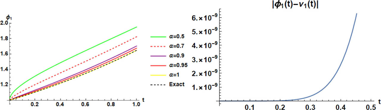
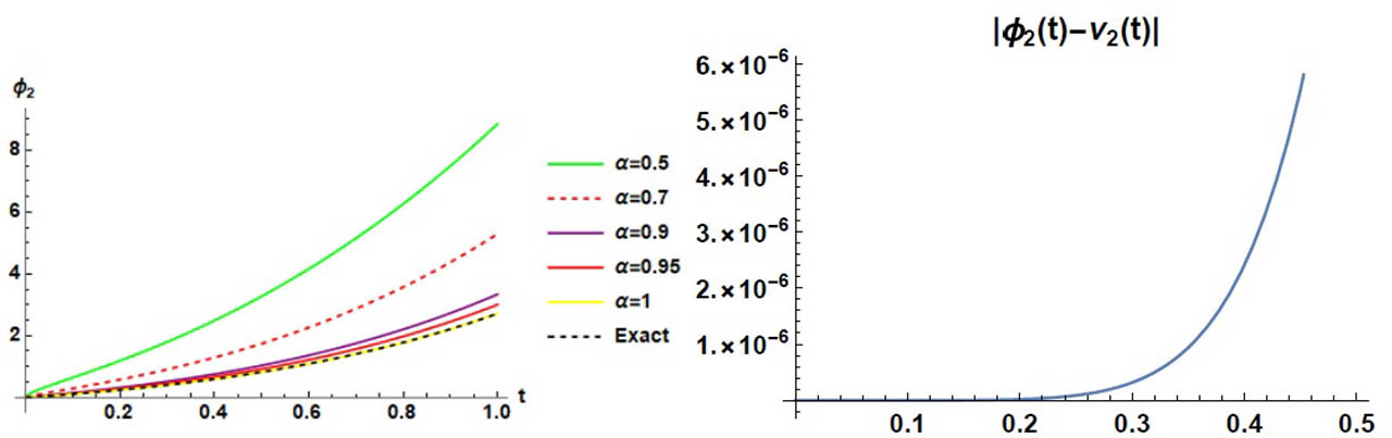
Exact, profile approximate solutions and absolute error regarding ν₂ of Example 1.

On the other side, as shown in Table 1, we provide numerical investigations on the accuracy of LRPS applied to Example 1. While as, in Table 2, we present the impact of the fractional order α acting on the values of the unknowns field functions ν_i(t) : i = 1, 2.

Table 1

Numerical values of φ₁(t) and φ₂(t) for α = 0.5, 0.7, 0.9 to Example 1.

t	α = 0.5		α = 0.7		α = 0.9
t	ν₁(t)	ν₂(t)	ν₁(t)	ν₂(t)	ν₁(t)	ν₂(t)
0.2	1.312141902	1.184140706	1.201599157	0.580240824	1.130764596	0.320222598
0.4	1.486564677	2.444376604	1.354985531	1.290827616	1.259270690	0.756805142
0.6	1.6445934256	4.006862318	1.506375497	2.249749087	1.396080779	1.365217628
0.8	1.7972927210	5.900827955	1.661915587	3.516856974	1.543797927	2.198213783

Table 2

Absolute errors: |φ₁(t) − ν₁(t)| and |φ₂(t) − ν₂(t)| to Example 1.

t	\|φ₁(t) − ν₁(t)\|	\|φ₂(t) − ν₂(t)\|
0.2	1.408981153×10⁻⁹	5.516320339×10⁻⁷
0.4	9.149350321×10⁻⁸	3.65457231×10⁻⁵
0.6	1.057576003×10⁻⁶	4.31280234×10⁻⁴
0.8	6.030974603×10⁻⁶	2.51274279×10⁻³

3.2 Example 2

Let us consider the following 3 × 3 nonlinear autonomous system [9, 10]

(31) {Dαν1(t)=ν1(t),Dαν2(t)=2(ν1(t))2,Dαν3(t)=3ν1(t)ν2(t);

subject to

(32) ν1(0)=1,ν2(0)=1,ν3(0)=0.

Apply the Laplace transform to (31)–(32), we get

(33) V1(s)=1s+V1(s)sα,V2(s)=1s+2sα(ℒ[ℒ−1[V1(s)]2]),V3(s)=3ℒ[ℒ−1[V1(s)]ℒ−1[V2(s)]]sα,

Assume that V₁(s), V₂(s) and V₃(s) have fractional power series as

(34) V1(s)=∑n=0∞ansnα+1,V2(s)=∑n=0∞bnsnα+1,V3(s)=∑n=0∞cnsnα+1,

with the k-th truncated series

(35) V1k(s)=∑n=0kansnα+1=1s+∑n=1kansnα+1,V2k(s)=∑n=0kbnsnα+1=1s+∑n=1kbnsnα+1,V3k(s)=∑n=0kcnsnα+1=∑n=1kcnsnα+1, respectively,

whose the Laplace residual functions for V1k(s) , V2k(s) and V3k(s) are

(36) LRes1(s)=V1(s)−1s−V1(s)sα,LRes2(s)=V2(s)−1s−1sα(ℒ[ℒ−1[V1(s)]2]),LRes3(s)=V3(s)−3ℒ[ℒ−1[V1(s)]ℒ−1[V2(s)]]sα.

Accordingly, the k-th Laplace residual functions, LRes^k, are

(37) LRes1k(s)=V1k(s)−1s−V1k(s)sα,LRes2k(s)=V2k(s)−1s−1sα(ℒ[ℒ−1[V1k(s)]2]),LRes3k(s)=V3k(s)−3ℒ[ℒ−1[V1k(s)]ℒ−1[V2k(s)]]sα,

To determine a₁, b₁ and c₁, we substitute (35) in (37) with k = 1 to get

(38) LRes11(s)=a1sα+1−1sα(1s+a1sα+1),LRes21(s)=b1sα+1−1sα(ℒ[ℒ−1[1s+a1sα+1]2]),LRes31(s)=c1sα+1−3sα(ℒ[ℒ−1[1s+a1sα+1]ℒ−1[1s+b1sα+1]]),

Multiply (38) by s^α⁺¹,

(39) sα+1LRes11(s)=a1−(1+a1sα),sα+1LRes21(s)=b1−s(ℒ[ℒ−1[1s+a1sα+1]2]),sα+1LRes31(s)=c1−3s(ℒ[ℒ−1[1s+a1sα+1]ℒ−1[1s+b1sα+1]]).

It is clear that when we solve lims→∞(sα+1LResm1(s))=0 , m = 1, 2, 3, we directly obtain

(40) a1=1,b1=2,c1=3.

Similarly, when we substitute (35) in (37) with k = 2 and then use the fact that lims→∞(sα+1LResm2(s))=0 , m = 1, 2, 3, we reach

(41) a2=1,b2=4,c2=9.

Hence, the 2^nd-approximate LRPS solution of V12(s) , V22(s) and V32(s) are

(42) V12(s)=1s+1sα+1+1s2α+1,V22(s)=1s+2sα+1+4s2α+1,V32(s)=3sα+1+9s2α+1.

Proceeding as the above illustrated steps in determining the unknown functions a_k, b_k and c_k, one can easily verify the following results:

(43) a3=1,a4=1,a5=1,

(44) b3=4+2Γ(1+2α)Γ2(1+α),b4=4+4Γ(1+3α)Γ(1+α)Γ(1+2α),b5=4+2(1Γ2(1+2α)+2Γ(1+α)Γ(1+3α))Γ(1+4α),

(45) c3=15+6Γ(1+2α)Γ2(1+α),c4=15+6(Γ2(1+2α)+3Γ(1+α)Γ(1+3α))Γ2(1+α)Γ(1+2α),c5=3(5+4Γ(1+4α)Γ2(1+2α)+2Γ(1+2α)Γ(1+4α)Γ3(1+α)Γ(1+3α)+1Γ(1+α)(4Γ(1+3α)Γ(1+2α)+6Γ(1+4α)Γ(1+3α))).

Therefore,

(46) V1(s)=1s+1sα+1+1s2α+1+1s3α+1+1s4α+1+1s5α+1+...,V2(s)=1s+2sα+1+4s2α+1+1s3α+1(4+2Γ(1+2α)Γ(1+α)2)+1s4α+1(4+4Γ(1+3α)Γ(1+α)Γ(1+2α))+1s5α+1(4+2(1Γ(1+2α)2+2Γ(1+α)Γ(1+3α))Γ(1+4α))+...,V3(s)=3sα+1+9s2α+1+1s3α+1(15+6Γ(1+2α)Γ(1+α)2)+1s4α+1(15+6(Γ(1+2α)2+3Γ(1+α)Γ(1+3α))Γ(1+α)2Γ(1+2α))+3(5+4Γ(1+4α)Γ(1+2α)2+2Γ(1+2α)Γ(1+4α)Γ(1+α)3Γ(1+3α)+1Γ(1+α)(4Γ(1+3α)Γ(1+2α)+6Γ(1+4α)Γ(1+3α)))s5α+1+... .

Consequently, the solution of (31)–(32) is

(47) ν1(t)=1+tαΓ(1+α)+t2αΓ(1+2α)+t3αΓ(1+3α)+t4αΓ(1+4α)+t5αΓ(1+5α)+...,ν2(t)=1+4t2αΓ(1+2α)+4t3αΓ(1+3α)+2t3αΓ(1+2α)Γ(1+α)2Γ(1+3α)+2tα+4t4αΓ(1+3α)Γ(1+2α)Γ(1+4α)Γ(1+α)+4t4αΓ(1+4α)+1Γ(1+5α)(t5α(4+2(1Γ(1+2α)2+2Γ(1+α)Γ(1+3α))Γ(1+4α)))+...,ν3(t)=tα(3(tα(3Γ(1+2α)+5tα(1Γ(1+3α)+tαΓ(1+4α)))+1Γ(1+α)2(2t2αΓ(1+2α)(1Γ(1+3α)+1Γ(1+4α)))+1+6t3αΓ(1+3α)Γ(1+2α)Γ(1+4α)Γ(1+α)))+... .

It is worth mentioning that the exact solutions to the system in Example 2 for the case α = 1 are ν₁(t) = e^t, ν₂(t) = e^2t and ν₃(t) = e^3t − 1 [9, 10]. We consider ψ1(t)=∑i=06aitiα to be the LRPS approximation of ν₁(t), ψ2(t)=∑i=06bitiα to be the LRPS approximation of ν₂(t) and ψ3(t)=∑i=06citiα to be the LRPS approximation of ν₃(t). In Figure 3, the first sub-figure represents the values of ψ₁(t) for different values of the fractional order α and values of ν₁(t), while the second sub-figure represents the absolute error |ν₁(t)− ψ₁(t)| when α = 1. In Figure 4, the first sub-figure represents the values of ψ₂(t) for different values of the fractional order α and values of ν₂(t), while the second sub-figure represents the absolute error |ν₂(t) − ψ₂(t)| when α = 1. In Figure 5, the first sub-figure represents the values of ψ₃(t) for different values of the fractional order α and values of ν₃(t), while the second sub-figure represents the absolute error |ν₃(t) − ψ₃(t)| when α = 1. For this 3 × 3 system, one can observe the same findings depicted for Example 1. Finally, as shown in Table 3, we provide numerical investigations on the accuracy of LRPS applied to Example 2.

Figure 3

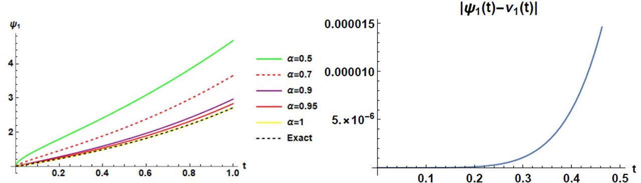
Exact, profile approximate solutions and absolute error regarding ν₁ of Example 2.

Figure 4

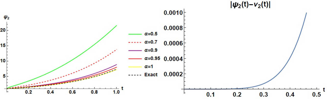
Exact, profile approximate solutions and absolute error regarding ν₂ of Example 2.

Figure 5

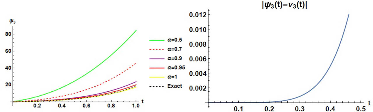
Exact, profile approximate solutions and absolute error regarding ν₃ of Example 2.

Table 3

t	\|ψ₁(t) − ν₁(t)\|	\|ψ₂(t) − ν₂(t)\|	\|ψ₃(t) − ν₃(t)\|
0.2	9.149350315×10⁻⁸	6.030974603×10⁻⁶	7.080039050 ×10⁻⁵
0.4	6.030974603×10⁻⁶	4.102618258×10⁻⁴	4.980922736 ×10⁻³
0.6	7.080039050×10⁻⁵	4.980922736×10⁻³	6.278346441 ×10⁻²
0.8	4.102618258×10⁻⁴	2.991775772×10⁻²	3.932243806 ×10⁻¹

4 Conclusion

A combination of two schemes; the Laplace transform and the residual power series, is adapted to solve nonlinear Caputo-fractional autonomous dynamical systems. The methodology, reliability and the accuracy of the new technique are introduced by solving 2 × 2 and 3 × 3 systems. The role of the fractional derivative is investigated by using graphical analysis. Finally, the advantage of the current method was depicted as converting the whole fractional problem into pure algebraic computational scheme which can be executed using any available computational softwares.

As a future work, the authors plan to extend the use of LRPS to solve multi-dimensional various fractional problems arising in Engineering and Science.

Funding information: The authors state no funding involved.
Author contributions: All authors have accepted responsibility for the entire content of this manuscript and approved its submission.
Conflict of interest: The authors state no conflict of interest.

References

[1] Almeida R, Guzowska M, Odzijewicz T. A remark on local fractional calculus and ordinary derivatives. Open Math. 2016;14:1122–1124.10.1515/math-2016-0104Search in Google Scholar

[2] Razzaghi M, Ordokhani Y. Solution of nonlinear Volterra- Hammerstein integral equations via rationalized Haar functions. Mathe. Probl. Eng. 2001;7(2):205–219.10.1155/S1024123X01001612Search in Google Scholar

[3] Owolabi KM, Hammouch Z. Spatiotemporal patterns in the Belousov-Zhabotinskii reaction systems with Atangana-Baleanu fractional order derivative. Phys. A: Stat. Mech. Appl. 2019;523:1072–1090.10.1016/j.physa.2019.04.017Search in Google Scholar

[4] Keshavarz E, Ordokhani Y, Razzaghi M. A numerical solution for fractional optimal control problems via Bernoulli polynomials. J. Vib. Control. 2016;22(18):3889–3903.10.1177/1077546314567181Search in Google Scholar

[5] Ejlali N, Hosseini SM, Yousefi SA. B-spline spectral method for constrained fractional optimal control problems. Mathe. Methods Appl. Sci. 2018;41(14):5466–5480.10.1002/mma.5090Search in Google Scholar

[6] Ganji RM, Jafari H. A new approach for solving nonlinear Volterra integro-differential equations with Mittag-Leffler kernel. Proc. Inst. Mathe. Mech. 2020;46(1):144–158.10.29228/proc.24Search in Google Scholar

[7] Jafari H, Firoozjaee MA, Johnston SJ. An effective approach to solve a system fractional differential equations. Alexandria Engineering Journal. 2020;59(5):3213–3219.10.1016/j.aej.2020.08.015Search in Google Scholar

[8] Dixit S, Singh O, Kumar S. An analytic algorithm for solving system of fractional differential equations. Journal of Modern Methods in Numerical Mathematics. 2010;1(1):12–26.10.20454/jmmnm.2010.25Search in Google Scholar

[9] Zurigat M, Momani S, Odibat Z, Alawneh A. The homotopy analysis method for handling systems of fractional differential equations. Applied Mathematical Modelling. 2010;34(1):24–35.10.1016/j.apm.2009.03.024Search in Google Scholar

[10] Wu XY, Xia JL. Two low accuracy methods for stiff systems. Applied mathematics and computation. 2001;123(2):141–153.10.1016/S0096-3003(00)00010-2Search in Google Scholar

[11] Eriqat T, El-Ajou A, Oqielat MN, Al-Zhour Z, Momani S. A new attractive analytic approach for solutions of linear and nonlinear Neutral fractional Pantograph equations. Chaos, Solitons & Fractals. 2020;138:109957.10.1016/j.chaos.2020.109957Search in Google Scholar

[12] Alquran M, Ali M, Alsukhour M, Jaradat I. Promoted residual power series technique with Laplace transform to solve some time-fractional problems arising in physics. Results in Physics. 2020;19:103667.10.1016/j.rinp.2020.103667Search in Google Scholar

[13] Ali M, Alquran M, Jaradat I. Asymptotic-sequentially solution style for the generalized Caputo time-fractional Newell-Whitehead-Segel system. Advances in Difference Equations. 2019;2019:70.10.1186/s13662-019-2021-8Search in Google Scholar

[14] Dehghan M, Manafian J, Saadatmandi A. Solving nonlinear fractional partial differential equations using the homotopy analysis method. Numerical Methods for Partial Differential Equations. 2010;26:448–479.10.1002/num.20460Search in Google Scholar

[15] Ganjiani M. Solution of nonlinear fractional differential equations using Homotopy analysis method. Appl. Math. Model. 2010;34:1634–1641.10.1016/j.apm.2009.09.011Search in Google Scholar

[16] Alquran M, Jaradat I. Delay-asymptotic solutions for the time-fractional delay-type wave equation. Physica A: Statistical Mechanics and its Applications. 2019;527:121275.10.1016/j.physa.2019.121275Search in Google Scholar

[17] Alquran M. Analytical solution of time-fractional two-component evolutionary system of order 2 by residual power series method. Journal of Applied Analysis and Computation. 2015;5(4):589–599.10.11948/2015046Search in Google Scholar

[18] He JH. Homotopy perturbation method: a new nonlinear analytical technique. Appl. Math. Comput. 2003;135:73–79.10.1016/S0096-3003(01)00312-5Search in Google Scholar

[19] Ali M, Alquran M, Jaradat I, Abu Afouna N, Baleanu D. Dynamics of integer-fractional time-derivative for the new two-mode Kuramoto-Sivashinsky model. Rom. Rep. Phys. 2020;72(1):103.Search in Google Scholar

[20] Alquran M, Jaradat I, Momani S, Baleanu D. Chaotic and soli-tonic solutions for a new time-fractional two-mode Kortewegde Vries equation. Rom. Rep. Phys. 2020;72(3):117.Search in Google Scholar

[21] Abu Irwaq I, Alquran M, Jaradat I, Noorani MSM, Momani S, Baleanu D. Numerical investigations on the physical dynamics of the coupled fractional Boussinesq-Burgers system. Romanian Journal of Physics. 2020;65(5–6):111.Search in Google Scholar

[22] Jaradat I, Al-Dolat M, Al-Zoubi K, Alquran M. Theory and applications of a more general form for fractional power series expansion. Chaos Solitons Fract. 2018;108:107–110.10.1016/j.chaos.2018.01.039Search in Google Scholar

[23] Jaradat I, Alquran M, Al-Dolat M. Analytic solution of homogeneous time-invariant fractional IVP. Adv. Differ. Equ. 2018;2018:143.10.1186/s13662-018-1601-3Search in Google Scholar

[24] Abu Irwaq I, Alquran M, Ali M, Jaradat I, Noorani MSM. Attractive new fractional-integer power series method for solving singulary perturbed differential equations involving mixed fractional and integer derivatives. Results in Physic. 2021;20:103780.10.1016/j.rinp.2020.103780Search in Google Scholar

[25] Jaradat I, Alquran M, Abdel-Muhsen R. An analytical framework of 2D diffusion, wave-like, telegraph, and Burgers’ models with twofold Caputo derivatives ordering. Nonlinear Dynamics. 2018;93(4):1911–1922.10.1007/s11071-018-4297-8Search in Google Scholar

[26] Alquran M, Al-Khaled K, Sivasundaram S, Jaradat HM. Mathematical and numerical study of existence of bifurcations of the generalized fractional Burgers-Huxley equation. Nonlinear Studies. 2017;24(1):235–244.Search in Google Scholar

[27] El-Ajou A, Abu Arqub O, Al-Smadi M. A general form of the generalized Taylor's formula with some applications. Appl. Math. Comput. 2015;256:851–859.10.1016/j.amc.2015.01.034Search in Google Scholar

[28] Komashynska I, Al-Smadi M, Abu Arqub O, Momani S. An efficient analytical method for solving singular initial value problems of nonlinear systems. Appl. Math. Inf. Sci. 2016;10(2):647–656.10.18576/amis/100224Search in Google Scholar

[29] Alquran M, Yousef F, Alquran F, Sulaiman TA, Yusuf A. Dualwave solutions for the quadratic-cubic conformable-Caputo time-fractional Klein-Fock-Gordon equation. Mathematics and Computers in Simulation. 2021;185:62–76.10.1016/j.matcom.2020.12.014Search in Google Scholar

Received: 2021-04-30

Accepted: 2021-08-03

Published Online: 2021-10-08

This work is licensed under the Creative Commons Attribution 4.0 International License.

Articles in the same Issue

https://doi.org/10.1515/nleng-2021-0022

Keywords for this article

Caputo-fractional autonomous nonlinear systems; Laplace transform; residual power series method

Creative Commons

BY 4.0