
Heat and Mass Transfer of Temperature-Dependent Viscosity Models in a Pipe: Effects of Thermal Radiation and Heat Generation
-
Fayyaz Ahmad

 ,
Mubashara Saeed
,
Mubashara Saeed

Abstract
In this paper, a study of the flow of Eyring-Powell (EP) fluid in an infinite circular long pipe under the consideration of heat generation and thermal radiation is considered. It is assumed that the viscosity of the fluid is an exponential function of the temperature of the fluid. The flow of fluid depends on many variables, such as the physical property of each phase and shape of solid particles. To convert the given governing equations into dimensionless form, the dimensionless quantities have been used and the resultant boundary value problem is solved for the calculation of velocity and temperature fields. The analytical solutions of velocity and temperature are calculated with the help of the perturbation method. The effects of the fluidic parameters on velocity and temperature are discussed in detail. Finite difference method is employed to find the numerical solutions and compared with the analytical solution. The magnitude error in velocity and temperature is obtained in each case of the viscosity model and plotted against the radius of the pipe. Graphs are plotted to describe the influence of various parameter EP parameters, heat generation parameter and thermal radiation parameters against velocity and temperature profiles. The fluid temperature has decreasing and increasing trends with respect to radiation and heat generations parameters, respectively.
1 Introduction
The study of non-Newtonian fluids has increased due to a substantial variety of engineering, industrial and commercial manufacturing applications. The study of Newtonian fluids is easy as compared to non-Newtonian fluids due to simple developed equations which can be handled numerically or analytically. The reason is that of a linear relationship between the rate of stress and strain in the case of Newtonian fluid, but this relation is not any more linear for non-Newtonian fluids. Various authors showed the applications of non-Newtonian fluids in their studies. Some significant examples of non-Newtonian fluids are cream, plastic melts, soap slurries, wet beach sand, mayonnaise, paper pulp, etc. [1]. Navier-Stokes equation is used to describe the flow behaviour of Newtonian fluid but there is no single equation to describe the flow behaviour of the non-Newtonian fluids with all the properties. Due to this reason, various empirical and semi-empirical non-Newtonian equations or models have been presented and used.
Ali et al. [2] studied an Eyring-Powell (EP) fluid under the effects of temperature-dependent viscosity cases in a pipe. They first convert their dimensional forms of momentum and energy equations with boundary conditions into non-dimensional form, and then discuss Reynolds and Vogel models for both momentum and energy equations. In their research work, they solved their equations with the help of both perturbation and numerical methods that match well. The flow of magnetohydrodynamics (MHD) EP nanofluid over an inclined surface is analysed by Khan et al. [3]. During their study, they assumed that the flow of fluid is incompressible and the fluid viscosity is varying exponentially. They expressed their results in the form of velocity and temperature profiles along with different parameters by plotting graphs and also in tabular form. Ellahi [4] examined the study of non-Newtonian nanofluid in the pipe and depicted the effects of magnetic and temperature-dependent viscosity. Akinshilo and Olaye [5] also analysed the flow of EP fluid in a pipe. They discussed the internal heat flow and temperature-dependent viscosity in their work. They solved the non-linear ordinary equation by using perturbation technique and examined the effect of fluidic parameters on velocity and temperature profiles. Akinbowale [6] studied the non-Newtonian flow of third-grade fluid in the horizontal channel. He solved an ordinary differential equation by using Adomian decomposition method and discussed the Vogel model for temperature-dependent viscosity and concluded that velocity distribution increases by decreasing the porosity parameter. Ellahi and Riaz [7] captured the magnetic effects in the flow of third-grade fluid in a pipe by taking variable viscosity. To calculate the analytical solution, the homotopy analysis method (HAM) was used. Aksoy and Pakdemirli [8] considered the non-Newtonian fluid with a porous medium between two parallel plates. They calculated the solutions of the non-linear differential equations by employing the perturbation technique. Three viscosity dependent cases were discussed i.e., (a) constant viscosity case; (b) Reynolds model; and (c) Vogel’s model. The validity range of the solution was also provided. Ellahi et al. [9] examined the third-grade fluid between the concentric cylinders and checked the effect of slip over this fluid. They discussed two cases, in the first one the outer cylinder is stationary and inner cylinder move and the second one the outer cylinder is moving and the inner cylinder is at rest position. They calculate the solutions for both conditions (with and without slip parameter). The flow of non-isothermal Poiseuille fluid was also examined by Farooq et al. [10]. They considered the fluid is flowing between two heated parallel inclined plates using coupled stress fluid which was incompressible. Perturbation techniques were used to calculate analytical solutions. In their paper, they discussed the Reynold’s model and obtained the expressions for temperature, velocity, dynamic pressure, shear stress and volume flow rate. Alharbi et al. [11] evaluated the effects of entropy generation in MHD EP fluid. They assumed that the flow is flowing over an oscillating porous stretching sheet and further assumed that the flow is unsteady. They analysed the behaviour of the heat source and thermal radiation in their study. They captured the effects of pertinent parameters on entropy generation rate, temperature, and velocity fields. They solved the governing equation by using HAM. The radiative effect on three-dimensional MHD flow of an EP fluid was described by Hayat et al. [12]. They calculated the series solution by non-linear analysis and also calculate the exact solution of the problem. Yurusoy [13] presented the heat transfer effects of third-grade fluid between two concentric cylinders. During his study, he considered that the fluid temperature is lower than the pipe temperature. He calculated the solution by using perturbation technique and discussed Reynolds model. Hayat et al. [14] explored the effect of porous medium of third-grade fluid. They solved the governing momentum and energy equations by employing HAM. They analysed the shear stress and velocity field at the plate. Massoudi and Christie [15] analysed the viscous dissipation and variable viscosity effects of third-grade fluid in a pipe and considered that the temperature of the fluid is lower than the temperature of the pipe. Huang [16] studied the heat generation effect of non-Newtonian fluid over a vertical permeable cone in a porous medium. The author used the Keller box method to find a solution of his problem and discussed the physical aspects of the problem. Analysis of EP nanofluid is selected by Hayat et al. [17]. They captured the effect of MHD flow over the non-linear stretching sheet and discussed the results for concentration and temperature profiles. Hayat and Nadeem [18] studied the three-dimensional flow of EP fluid and discussed the heat flux and mass quantities. They discussed the behaviour of temperature and Cattaneo-Christov heat flux theory.
From the above-cited studies, it is noted that there is no study available in literature to capture the effects of radiative heat flux and heat generation on EP fluid in a circular long pipe under various models of the viscosities. The considered fluid model (EP) is much complex and is advantageous over a Power-law model due to two aspects. The first one is that this model is not driven from an empirical relation like a Power-law model. The second one is, this fluid model can be reduced into a Newtonian fluid model for the low and high shear rates.Therefore, the objective of our investigation is to obtain the numerical and perturbation solutions of the one-dimensional flow of an EP fluid in a pipe under the combined effects of radiative and heat absorption. As various engineering processes only happen at moderate temperature, so the consideration of radiative heat flux cannot be ignored in these kind of processes namely space vehicles, gas turbines, propulsion devices, and nuclear plants [19], [20]. Futher, the study of heat generation (or absorption) in moving fluid is useful in the problems of chemical reaction. The flows in the porous media have numerious applications like, oil reservoir and geothermal [21], [22]. The absolute error in velocity and temperature will be presented. Three famous models will discuss which are listed below.
Constant viscosity model
Reynolds model
Vogel’s model
The numerical solution for all above-mentioned viscosity models will be obtained by the finite-difference method in our study. The effects of various physical parameters on viscosity and temperature profiles will be highlighted together with the validity of the perturbation solution. The current study can be useful to increase the heat transfer processes in energy conservation, medical process, fuel cells and micro-mixing. The applications of this problem are also beneficial in heat exchangers, film flow, catalytic reactors, paper production and polymer solutions. This study will be helpful in future to investigate the behaviour of velocity and temperature fields against pertinent prameters, whenever preliminary data of EP model is given.
2 Formulation of the Problem
Let us consider the one-dimensional, steady-state flow of non-Newtonian fluid in a pipe with the account of effects of radiation and heat generation. It is assuming that the flow is flowing due to applied pressure gradient and the viscosity is a function of temperature. The systematic flow behaviour is shown in Figure 1.
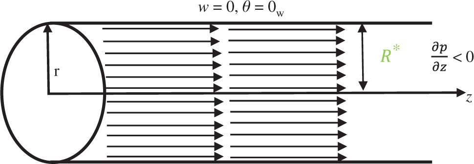
Geometry of the flow problem.
The velocity and temperature fields for the present problem are defined by
The Cauchy stress tensor T[23], [24] is
where p is the pressure, I is the identity element. Now for the current situation, the extra stress tensor S is defined as
where
and
As
with the help of (10), we get
Putting these values in (4), (4) takes the following form:
Using
Now by substituting the value of A1 in (15), we get
where S is defined as
Now using the value of S in (16)
From the above (18), only two components of extra stress are left which are:
The general form of the equation of motion in cylindrical coordinates system is:
Due to steady-state flow, we have
As the velocity components u = 0 and v = 0 so, left-hand side of general equations will vanish and only right-hand side will survive which is given by:
As, in the current investigation, the flow is flowing along z-direction only (one dimensional) so we can use the simple derivative instead of partial derivative symbols.
where
Now for the derivation of the heat equation, first the general form of the heat equation is considered
The radiative heat flux HR [25], [26] for the current situation is defined by
To obtain the values of θ4, we will expand θ4 in the Taylor series expansion about θw and overlooking upper order terms, yields
Using the value of θ4 into (34), we have
Use (32), (33) and (34) into (31), we get
The boundary conditions for (29) and (37) are:
Now introducing the dimensionless quantities
The dimensionless equations are given by:
where
The dimensionless equations of motion and energy based on viscosity models are discussed in the next one.
3 Viscosity Models
Based on the viscosity of the fluid, three different models are selected. In the first case, viscosity is chosen as a constant i.e., viscosity does not depend on temperature and in second and third cases, viscosity is a function of fluid temperature and these models are known as Reynolds and Vogel’s models. In the last two models, viscosity is defined as an exponent form.
Constant Viscosity Model
For this case, we set
The new forms of the equation of motion and heat equation for the present case are:
(43)(44)(45)To solve (43)–(45), let us assume to apply perturbation expansion on momentum and energy equation.
(46)where ϵ is the perturbation parameter and (0 < ϵ ≤ 1). By separating each order of we have the following systems:
System of order (ϵ0) for velocity profile:
(47)(48)System or order (
(49)(50)System of order (ϵ0) for temperature profile:
(51)(52)System or order (ϵ1) for temperature profile:
(53)(54)By solving each order of ϵ, we have the following results for velocity profile:
(55)(56)Results for temperature profile:
(57)(58)The final expressions for temperature and velocity are:
(59)(60)Reynolds Model
For the case of variable viscosity model i.e., Reynolds model, we will set the values of viscosity in term of temperature as:
(61)In view of the above setting, the equation of motion and heat equation is defined by:
(62)(63)The perturbation expansions on momentum and energy equations for this case are as follows:
(64)System of order
(65)(66)System or order
(67)(68)System or order (ϵ0) for temperature profile:
(69)(70)System or order (
(71)(72)By solving each order of ϵ, we have the following results for velocity profile:
(73)(74)Results for temperature profile are:
(75)(76)The final expression for temperature and velocity are:
(77)(78)Vogel’s Model
For Vogel’s model, we take the values of viscosity as
With the help of the above substitution, we get the equation of motion and heat equation in the following form:
(79)where
The perturbation expansions for this case are as follows:
(80)System of order (ϵ0) for velocity profile:
(81)(82)System of order (ϵ0) for temperature profile:
(83)(84)System or order (
(85)(86)System or order (
(87)(88)By solving each order of ϵ, we have the following results for velocity and temperature profiles:
(89)(90)(91)(92)The final expression for temperature and velocity are as follows:
(93)(94)
4 Numerical Method
The perturbation solution is compared with the explicit finite difference approximated numerical solution. The discretisation of the given domain
where
where
Stencil for one-sided first-order derivative which is also second-order accurate is
The boundary condition at
or
The applications of above finite difference formulas to (40) and (41) provide the non-linear system of equations. To find the solution the resultant system, Newton method [27], [28], [29], [30], [31], [32], [33], [34], [35] is used.
Velociy and temperature profiles for Vogel’s viscosity model.
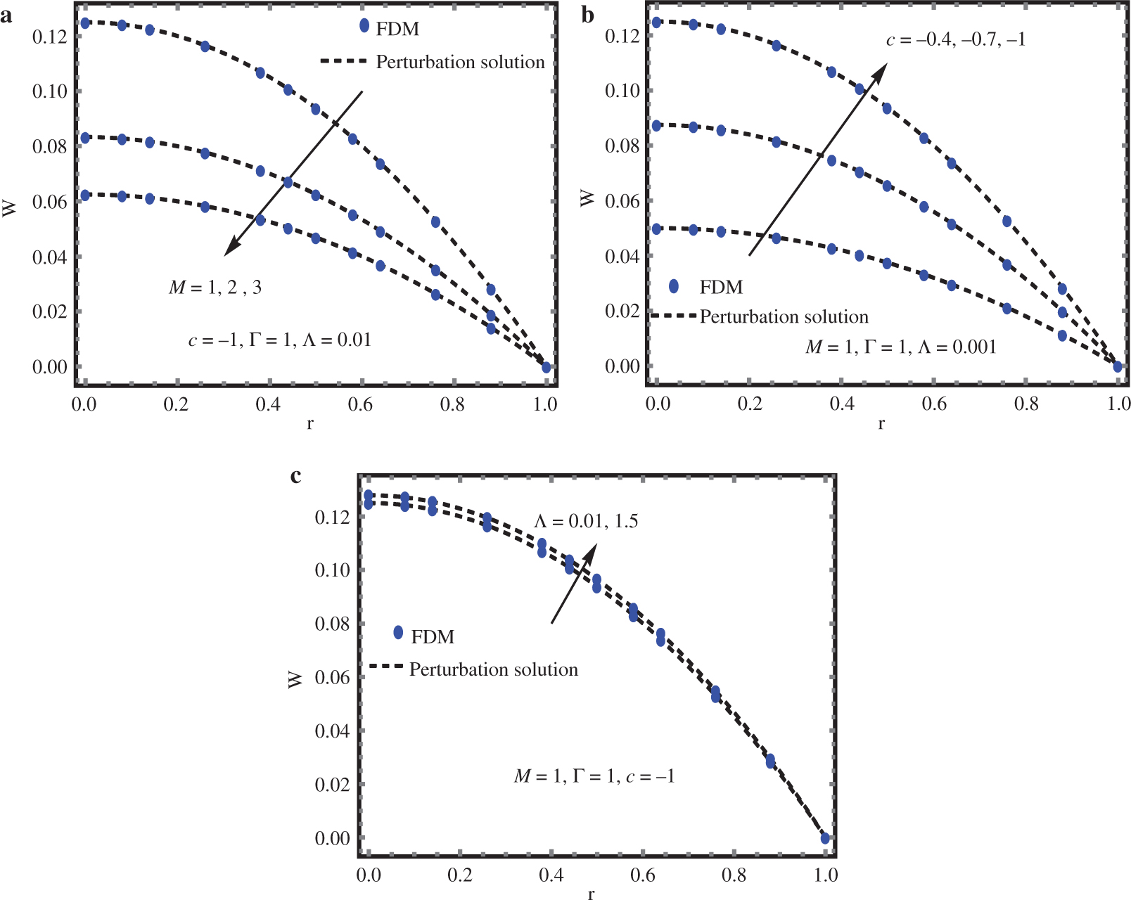
Effects of (a) Material parameter (M), (b) Pressure gradient parameter (c) and (c) non-Newtonian parameter (Γ) on velocity profile.
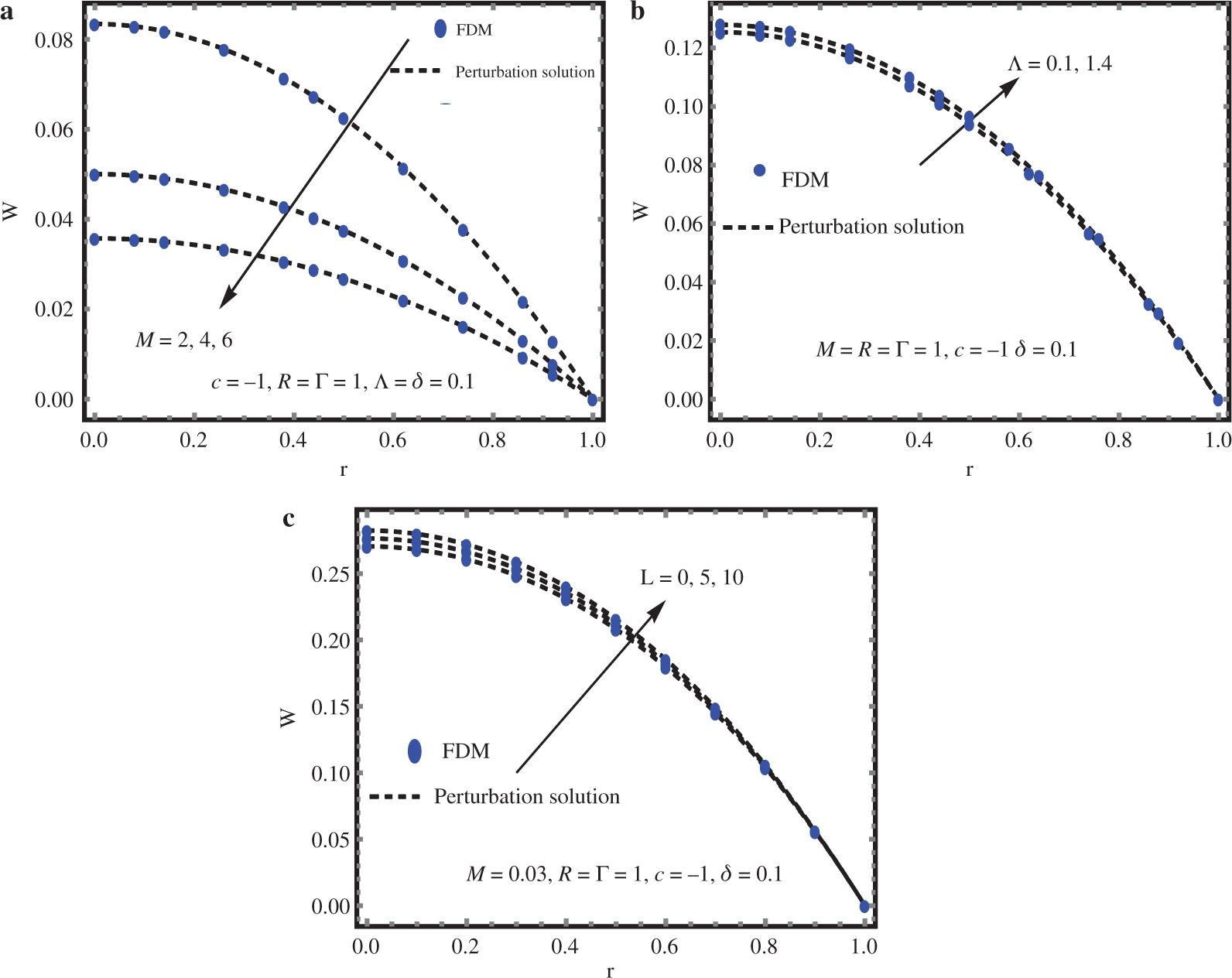
Effects of (a) Material parameter (M), (b) non-Newtonian parameter (Γ) and (c) Reynolds viscosity index (L) on velocity profile.
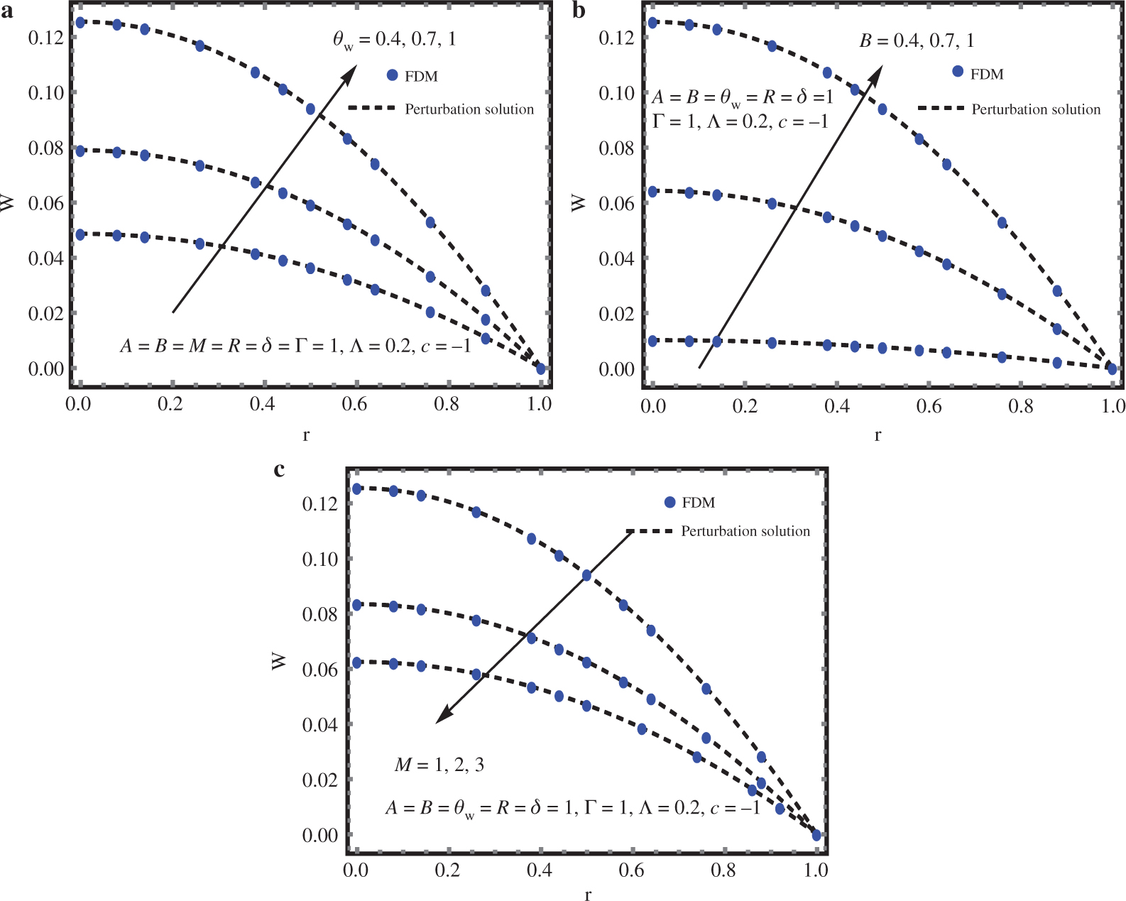
Effects of (a) Wall’s temperature (θw), (b) Vogel’s viscosity index and (c) Material parameter (M) on velocity profile.
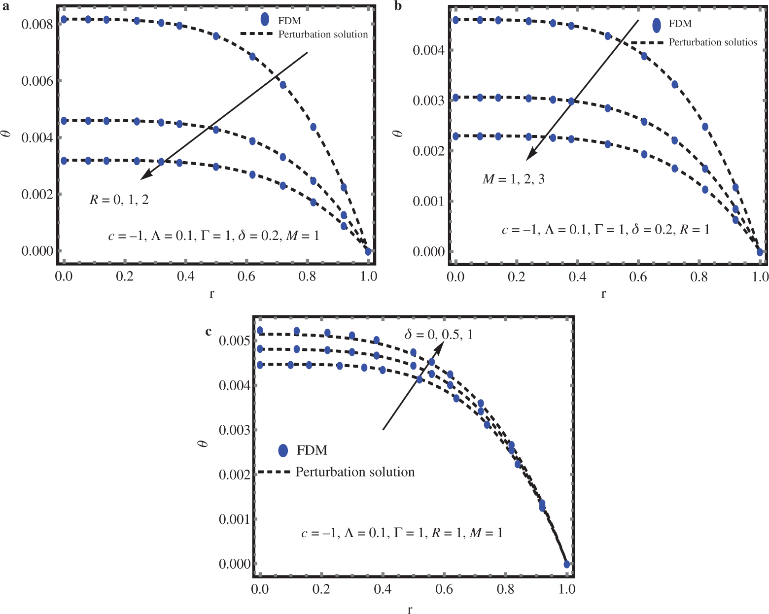
Effects of (a) Radiation parameter (R), (b) Material parameter (M) and (c) Heat generation parameter (δ) on temperature profile.
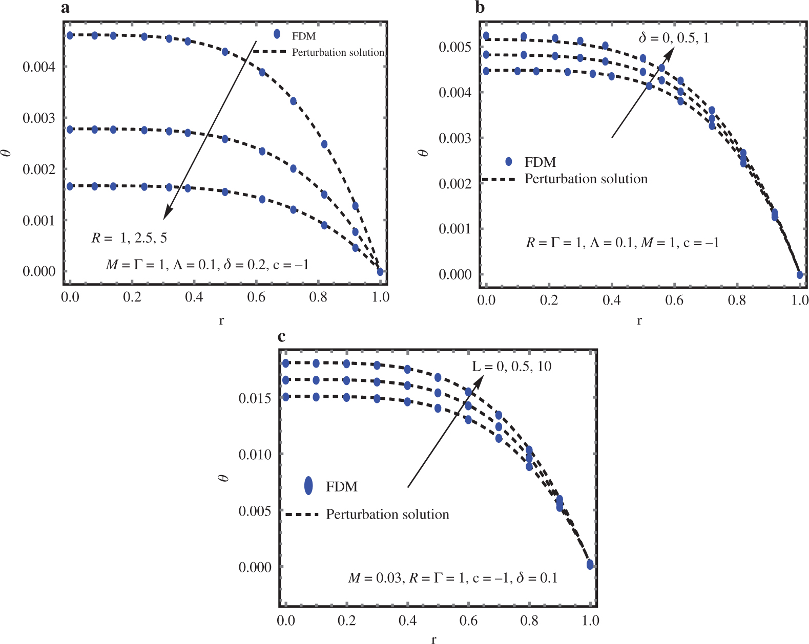
Effects of (a) Radiation parameter (R), (b) Heat generation parameter (δ) and (c) Reynolds viscosity index (L) on temperature profile.
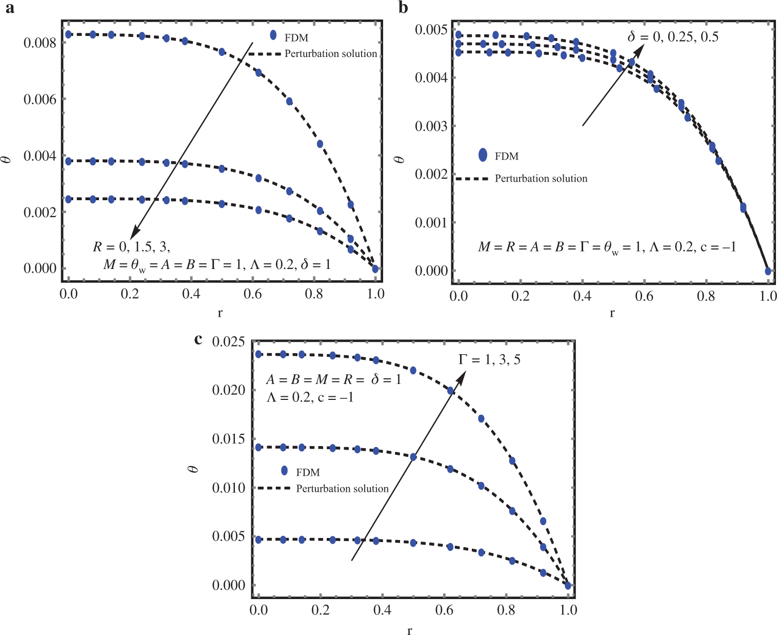
Effects of (a) Radiation parameter (R), Heat generation parameter (δ) and (c) Viscous dissipation parameter (Γ) on temperature profile.
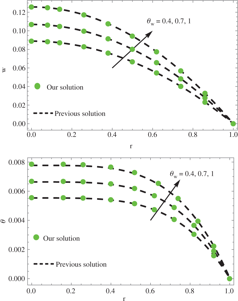
5 Comparison with Previous Study
Our explicit finite difference numerical code is validated with the solution of [2]. For this, we solved the direct non-dimensional system of equations with boundary conditions of [2] with the help of our numerical code. The reported the solution of an EP fluid [2] under the account of constant and variable properties of viscosity in a pipe without the absence of thermal radiation and heat generation. The numerical results are presented for Vogel’s viscosity model which are displayed in Figure 2 in term of velocity and temperature when
6 Results and Discussion
The basic purpose of the current section is to explain the physical aspects of the emerging parameters on the distributions of velocity and temperature by considering the flow of EP fluid in a long circular pipe. Three famous models on the basis of viscosity property i.e., constant viscosity model, Reynolds model, and Vogel’s model, respectively are discussed with the help of graphs.
To demonstrate the results of the given study, Figures 3–8 have been drawn. Figures 3–5 are related to the effects of different parameters on the velocity field, and Figures 6–8 display the effects of different parameters on the temperature field for all above-mentioned cases. These graphs exhibited the comparison of results of numerical solution and perturbation solution which are well agreed to each other. The results of the perturbation solution are represented by solid lines while the numerical solution is represented by a solid circle in each figure.
Absolute error between analytical and numerical solutions for the case of Reynolds viscosity model M = 1, c = −3, L = 1, Λ = 0.5, Γ = 10.
| R | δ | Perturbation Solution | Numerical Solution | Absolute Error | |||
|---|---|---|---|---|---|---|---|
| wmax | θmax | wmax | θmax | wE | θE | ||
| 2 | 1 | 0.43652 | 0.37130 | 0.49977 | 0.41889 | ||
| 3 | 1 | 0.42841 | 0.27183 | 0.47282 | 0.29605 | ||
| 4 | 1 | 0.42333 | 0.22923 | 0.45939 | 0.21403 | ||
| 5 | 0.4 | 0.41987 | 0.17051 | 0.45012 | 0.17899 | ||
| 5 | 0.7 | 0.41987 | 0.17344 | 0.45065 | 0.18293 | ||
| 5 | 1 | 0.41987 | 0.17637 | 0.45120 | 0.18702 | ||
6.1 Effects of Dimensionless Parameters on Velocity Profile
First, we discuss plots of velocity for the constant case. Figure 3a displays the effect of material parameter M on the velocity profile. We noticed that the velocity of the fluid decreases by increasing the value of material parameter M. The physical reason is that when we increase the values of M, the viscosity of the fluid also increases due to the direct relation between M and
6.2 Effects of Dimensionless Parameters on Temperature Profile
Here, Figures 6–8 are plotted to depict the effect of pertinent parameters on the temperature profile of all viscosity models. Figure 6a–c highlights the effect of radiation parameter
7 Error Magnitude
We compare the solutions obtained by the perturbation method and the explicit finite difference method. The absolute error in velocity and temperature distribution for the case of Reynolds viscosity model is listed in Table 1. From this table, it is noted that, the maximum absolute error in velocity and temperature is of the order of 10−2. This error increases with the increase in values of thermal radiation and heat generation parameters.
8 Conclusion
In this paper, we studied the combined effects of thermal radiation and heat generation in the one-dimensional flow of an EP fluid in a pipe. The dimensional governing momentum and energy equations are transformed into dimensionless form under the defined dimensionless quantities. In the present scenario, the viscosity is not only taken as a constant but it is also considered as a function of temperature namely Reynolds and Vogel’s models. The highly non-linear boundary value problem is solved with the perturbation method as well as the finite difference method. The perturbation method is used to obtain the analytical expressions of velocity and temperature in each case. For the validation of our analytical solution, the eminent finite difference method is to pick and solve the direct dimensionless equations under the prescribed boundary conditions of each case of viscosity model.
The results of this study reveal the following effects:
The velocity and temperature are decreasing functions of material parameter M.
The influence of c and Λ are same in case of velocity function.
The velocity is an increasing function of Vogel’s model parameter B and θw.
The temperature profile predcits the decreasing behaviour via material and radiation parameters and increment against heat generation parameter δ and viscous dissipation parameter Γ.
Solution benchmark [2]
Plots for velocity:
Constant case:
Reynolds model
Vogel’s model
Constant case (Temperature graphs)
Reynolds model
Vogel’s model
Nomenclature
Radius of pipe
- M
Material parameter
- 𝚲
Non-Newtonian parameter
- c
Pressure gradient parameter
- Q
Heat generation constant
- 𝜽m
Bulk means fluid temperature
- 𝝁
Viscosity of the fluid
- S
Cauchy’s stress tensor
- X, Y
Material constants
- A1
Rivlin-Ericksen tensor
- HR
Radiative heat flux
- k∗
Heat absorption parameter
- 𝜹
Heat genration parameter
- ŵ
Velocity components along z-direction
Dimensionless radius
- θ
Temperature of the fluid
Wall’s temperature
- k
Thermal conductivity
- w0
Reference velocity
- p
Pressure of the fluid
Viscosity of the fluid
- ϵ
Perturbation parameter
- Γ
Viscous dissipation parameter
- A, B
Vogel’s viscosity index
- L
Reynolds viscosity index
- R
Radiation parameter
Appendix
References
[1] T. Hayat, Z. Iqbal, M. Sajid, and K. Vajravelu, Int. Commun, Heat Mass Trans. 35, 1297 (2008).10.1016/j.icheatmasstransfer.2008.07.008Suche in Google Scholar
[2] N. Ali, F. Nazeer, and M. Nazeer, Z. Naturforsch. A 73, 265 (2018).10.1515/zna-2017-0435Suche in Google Scholar
[3] A. A. Khan, F. Zaib, and A. Zaman, J. Braz. Soc. Mech. Sci. Eng. 39, 5027 (2017).10.1007/s40430-017-0881-ySuche in Google Scholar
[4] R. Ellahi, Appl. Math. Model 37, 1451 (2013).10.1016/j.apm.2012.04.004Suche in Google Scholar
[5] A. T. Akinshilo and O. Olaye, J. King Saud Univ. Eng. Sci. 31, 271 (2017).10.1016/j.jksues.2017.09.001Suche in Google Scholar
[6] A. T. Akinbowale, Eng. Sci. Technol. Int. J. 20, 1602 (2017).Suche in Google Scholar
[7] R. Ellahi and A. Raiz, Math. Comp. Model. 52, 1783 (2010).10.1016/j.mcm.2010.07.005Suche in Google Scholar
[8] Y. G. Aksoy and M. Pakdemirli, Trans. Porous Media 83, 375 (2010).10.1007/s11242-009-9447-5Suche in Google Scholar
[9] R. Ellahi, T. Hayat, F. M. Mahomed, and S. Asghar, Nonlin. Anal. Real World Appl. 11, 139 (2010).10.1016/j.nonrwa.2008.10.051Suche in Google Scholar
[10] M. Farooq, M. T. Rahim, S. Islam, and A. M. Siddiqui, J. Assoc. Arab Univ. Basic Appl. Sci. 14, 9 (2013).10.1016/j.jaubas.2013.01.004Suche in Google Scholar
[11] S. O. Alharbi, A. Dawar, Z. Shah, W. Khan, M. Idrees, E. Appl. Sci. 8, 2588 (2018).10.3390/app8122588Suche in Google Scholar
[12] T. Hayat, M. Awais, and S. Asghar, J. Egyptian Math. Soc. 21, 379 (2013).10.1016/j.joems.2013.02.009Suche in Google Scholar
[13] M. Yurusoy, Math. Comp. Appl. 9, 11 (2004).10.3390/mca9010011Suche in Google Scholar
[14] T. Hayat, R. Naz, and S. Abbasbandy, Trans. Porous Media 87, 355 (2011).10.1007/s11242-010-9688-3Suche in Google Scholar
[15] M. Massoudi and I. Christie, Int. J. Non-Lin. Mech. 30, 687 (1995).10.1016/0020-7462(95)00031-ISuche in Google Scholar
[16] C. Huang, King Saud Univ. Eng. Sci. 30, 106 (2018).10.1016/j.jksus.2016.09.009Suche in Google Scholar
[17] T. Hayat, I. Ullah, A. Alsaedi, and M. Farooq, Results Phys. 7, 189 (2017).10.1016/j.rinp.2016.12.008Suche in Google Scholar
[18] T. Hayat and S. Nadeem, Results Phys. 7, 3910 (2017).10.1016/j.rinp.2017.09.048Suche in Google Scholar
[19] T. Hayat, S. Qayyum, S. A. Shehzad, and A. Alsaedi, Results Phys. 7, 562 (2017).10.1016/j.rinp.2016.12.009Suche in Google Scholar
[20] F. M. Abbasi, T. Hayat, B. Ahmad, and B. Chen, J. Cent. South Univ. 22, 2369 (2015).10.1007/s11771-015-2762-9Suche in Google Scholar
[21] G. M. Pavithra and B. J. Gireesha, J. Math. 2013, 583615 (2013).10.1155/2013/583615Suche in Google Scholar
[22] V. D. Marcello, A. Cammi, and L. Luzzi, Chem. Eng. Sci. 65, 1301 (2010).10.1016/j.ces.2009.10.004Suche in Google Scholar
[23] M. Nazeer, F. Ahmad, A. Saleem, M. Saeed, S. Naveed, et al., Z. Naturforsch. A 47, 961 (2019).10.1515/zna-2019-0095Suche in Google Scholar
[24] M. Nazeer, F. Ahmad, M. Saeed, A. Saleem, S. Khalid, et al., J. Braz. Soc. Mech. Sci. Eng. 41, 518 (2019).10.1007/s40430-019-2005-3Suche in Google Scholar
[25] N. Ali, M. Nazeer, T. Javed, and M. Razzaq, Eur. Phys. J. Plus 2, 134 (2019).10.1140/epjp/i2019-12448-xSuche in Google Scholar
[26] M. Nazeer, N. Ali, and T. Javed, J. Porous Media 21, 953 (2018).10.1615/JPorMedia.2018021123Suche in Google Scholar
[27] M. Nazeer, N. Ali, and T. Javed, Can. J. Phys. 96, 576 (2018).10.1139/cjp-2017-0639Suche in Google Scholar
[28] N. Ali, M. Nazeer, T. Javed, and M. A. Siddiqui, Heat Trans. Res. 49, 457 (2018).10.1615/HeatTransRes.2018019422Suche in Google Scholar
[29] M. Nazeer, N. Ali, and T. Javed, Int. J. Numer. Methods Heat Fluid Flow 28, 10, 2404 (2018).10.1108/HFF-10-2017-0424Suche in Google Scholar
[30] N. Ali, M. Nazeer, T. Javed, and F. Abbas, Meccanica 53, 3279 (2018).10.1007/s11012-018-0884-5Suche in Google Scholar
[31] M. Nazeer, N. Ali, T. Javed, and Z. Asghar, Eur. Phys. J. Plus 133, 423 (2018).10.1140/epjp/i2018-12217-5Suche in Google Scholar
[32] M. Nazeer, N. Ali, and T. Javed, Can. J. Phys. 97, 1 (2019).10.1139/cjp-2017-0904Suche in Google Scholar
[33] M. Nazeer, N. Ali, T. Javed, and M. Razzaq, Int. J. Hydrog. Energy 44, 953 (2019).10.1016/j.ijhydene.2019.01.236Suche in Google Scholar
[34] M. Nazeer, N. Ali, T. Javed, and M. W. Nazir, Eur. Phys. J. Plus 134, 204 (2019).10.1140/epjp/i2019-12562-9Suche in Google Scholar
[35] W. Ali, M. Nazeer, and A. Zeeshan, 10th International Conference on Computational & Experimental Methods in Multiphase & Complex Flow, 21–23 May 2019, Lisbon, Portugal.Suche in Google Scholar
©2020 Walter de Gruyter GmbH, Berlin/Boston
Artikel in diesem Heft
- Frontmatter
- Dynamical Systems & Nonlinear Phenomena
- Bifurcation Analysis for Small-Amplitude Nonlinear and Supernonlinear Ion-Acoustic Waves in a Superthermal Plasma
- Propagation of Waves in a Nonideal Magnetogasdynamics with Dust Particles
- Delta-Shock Solution to the Eulerian Droplet Model by Variable Substitution Method
- Solitary Wave with Quantisation of Electron’s Orbit in a Magnetised Plasma in the Presence of Heavy Negative Ions
- Heat and Mass Transfer of Temperature-Dependent Viscosity Models in a Pipe: Effects of Thermal Radiation and Heat Generation
- Solid State Physics & Materials Science
- Michelson Interferometric Hydrogen Sulfide Gas Sensor Based on NH2-rGO Sensitive Film
- Insight into the Structural, Electrical, and Magnetic Properties of Al-Substituted BiFeO3 Synthesised by the Sol–Gel Method
- Theoretical Studies of the Defect Structures for Cu(en)32+ and Ru(en)33+ Clusters in Tris(Ethylenediamine) Complexes
- Thermodynamics & Statistical Physics
- A Framework for Sequential Measurements and General Jarzynski Equations