1 Introduction

Lie symmetries are an essential tool for the study of nonlinear differential equations. The main characteristic of the Lie symmetry analysis is that invariant surfaces, in the space where the parameters of the nonlinear differential equation evolve, are determined, which can be used to perform an extended analysis of the nonlinear differential equation [1], [2], [3], [4], [5], [6], [7], construct conservation laws [8], [9], [10], and when it is feasible to determine solutions of the differential equation [11], [12], [13], [14]. In applied mathematics Lie symmetries cover a wide range of applications from physics, biology, financial mathematics, and many others (for instance, see [15], [16], [17], [18], [19], [20], [21], [22], [23], [24], [25], [26], [27], [28] and references therein).

In this work, we are interested on the application of Lie’s theory on a system of partial differential equations (PDEs) describing one-dimensional rotating shallow water phenomena. The system of our consideration expressed in Lagrangian coordinates is [29]:

where h=h(t,x) denotes the height of the fluid surface, u=u(t,x) denotes the velocity component in the x-direction, and v=v(t,x) is the other horizontal velocity component that is in the direction orthogonal to the x-direction [29]. Parameter γ is the polytropic parameter of the fluid, where in this work is assumed to be 0⩽γ. The system (1–3) is important for the study of atmospheric phenomena like geostrophic adjustment and zonal jets. For more details of the physical properties of the above system, we refer the reader in [30], [31], [32] and references therein.

The application of Lie symmetries in shallow-water theory is not new. Indeed, there are various studies in the literature [33], [34], [35], [36], [37], [38] that has provided important results with special physical interest. Recently, a detailed study of the nonlocal symmetries for a variable coefficient shallow water equation was performed in [39]. However, the majority of these studies are for the case where the fluid has a specific polytropic exponent γ, or the shallow water equations describe nonrotating phenomena. The plan of the article is as follows: In Section 2, we present the basic properties and definitions of Lie symmetry analysis, which is the main mathematical tool for our analysis. The main results of this work are presented in Section 3. More specifically, we reduce the system (1–3) into two equations for the variables h and v. We derive that the latter system of two PDEs admits five Lie point symmetries, and we study all the possible reductions in ordinary differential equations (ODEs) with the use of zero-order Lie invariants. We find that the reduced systems can be solved explicitly, and we derive the algebraic solution or closed-form solutions for every possible reduction and every value of the parameter γ. The latter result is important because it shows how powerful the method of Lie symmetry analysis is for the study of shallow-water phenomena to prove the existence of solutions for the model of our study. Emphasis is given on the travel-wave and scaling solutions. Finally, our discussion and conclusions are presented in Section 4.

2 Preliminaries

In this section, we briefly discuss the basic definitions and main steps for the determination of Lie point symmetries for differential equations.

Consider a system of PDEs

where u^Adenotes the dependent variables, yⁱ are the independent variables, and uiA=∂uA∂yi.

We assume the one-parameter point transformation (1PPT) in the space of the independent and dependent variables:

in which ε is an infinitesimal parameter; the differential equation (4) remains invariant if and only if

or equivalently [12]

The latter conditions is expressed

where ℒ denotes the Lie derivative with respect the vector field X[n], which is the n^th extension of generator X of the infinitesimal transformation (5, 6) in the jet space {yi,uA,u,iA,…}

with generator

and

When condition (9) is satisfied for a specific 1PPT, the vector field X is called a Lie point symmetry for the system of PDEs (4). For an unknown 1PPT, in order to specify the generators X, which are Lie point symmetries for a given differential equation, from the symmetry condition (9), we specify a system of PDEs with dependent variables in the components of the generator X. The solution of the latter system provides the generic symmetry vector, and the number of independent solutions gives the number of independent vector field and the dimension of the admitted Lie algebra.

3 Lie Symmetry Analysis

We write the system (1–3) as two second-order PDEs:

while the application of Lie’s theory provides a five-dimensional Lie algebra consists by the following vector fields:

In Table 1, the commutators of the Lie symmetries are presented. Consequently, from Table 1, we can refer that the admitted Lie algebra is the {2A1⊕s 2A1}⊕sA1 in the Morozov–Mubarakzyanov Classification Scheme [40], [41], [42], [43]. However, in the limit where γ = 1, the admitted Lie algebra is the 2A1⊕s 3A1.

In order to continue with the application of the Lie point symmetries, it is important to determine the one-dimensional optimal system and invariants [44]. In order to do that, the adjoint representations should be calculated. By definition, for every basis of the Lie symmetries X_i, the adjoint representation is given by the following expression:

For the admitted Lie point symmetries of the system (13, 14), the adjoint representation is given in Table 2. In order to find the optimal system, we consider the generic symmetry vector:

and we find the equivalent vectors by considering the adjoint representation. At this point, it is important to mention that the adjoint action admits two invariant functions, the ϕ1(ai)=a1 and ϕ2(ai)=a5 [45]. The invariants can be used to simplify the calculations on the derivation of the optimal system. Indeed, we have to consider the cases a1a2≠0 and a1a2=0.

Case 1: For a1a5≠0, we have that

becomes

for specific values of the parameters ε2,ε3 and ε₄.

Case 2: For a1a5=0, there are three subcases, (a) a₁ = 0, a5≠0; (b) a1≠0, a₅ = 0; and (c) a1=a5=0.

Case 2a: For a₁ = 0 and a2≠0, and following the steps as before, we find the optimal system X₅ where γ ≠ 1. In the limit, γ = 1, the generic optimal system is a3X3+a4X4+X5.

Case 2b: For a₁ = 0 and a1≠0, the optimal system is derived:

which for specific values of ε₃ and ε₄ is simplified as

Parameter a₂ is not an invariant; hence, it can be zero too. Hence, the two optimal systems are a1X1+a2X2 and X₁.

Case 2c: For a1=a5=0, we calculate the generic optimal systems a2X2+a3X3+a4X4.

Hence, the one-dimensional optimal systems for γ ≠ 1:

and for γ = 1:

There is a difference in the number of one-dimensional optimal systems, which depends on the parameter γ, which is expected because the structure of the Lie algebra changes.

We proceed our analysis by applying the Lie symmetries to reduce the system of PDEs into a system of ODEs and solve the resulting ODEs by applying the method of Lie symmetries.

3.3 Travel-Wave Solution

The linear combination of X₁ + cX₂ provides travel-wave solutions h=H(x−ct),v=V(x−ct) where parameter c describes the wave speed. The reduced system is

(20)Vξξ−H−2Hξ=0,

(21)c2Vξξ−Hγ−1Hξ+V=0.

in which the new independent parameter ξ is defined as ξ=x−ct.

From (20), we derive

(22)H−1=H0−Vξ,

where by substitute in (21) it follows

(23)(c2−(H0−Vξ)−γ−1)Vξξ+V=0.

The latter equation admits only one Lie point symmetry for γ ≽ 1, the autonomous symmetry ∂ξ. Recall that for γ=−1, (23) becomes a maximally symmetric equation, but such value for parameter γ is not physically accepted.

Application of the differential invariants of the autonomous symmetry vector ∂ξ in (23) leads to the nonlinear first-order ODE:

(24)w(H0−w)dwdz=z((H0−w)−γ−c2(H0−w))−1,

with solution

(25)γ(γ−1)(z2+c2w2+w0)+(H0−w)−γ+1=0,

where the new variables {z,w(z)} are defined as z=V(ξ) and w(z)=Vξ.

In the simplest case where the integration constant H₀ vanishes and γ = 1, the generic solution is given in terms of the Lambert function:

(26)ln(w(z))=−12W(−c2exp(z2+2w0))+z22+w0.

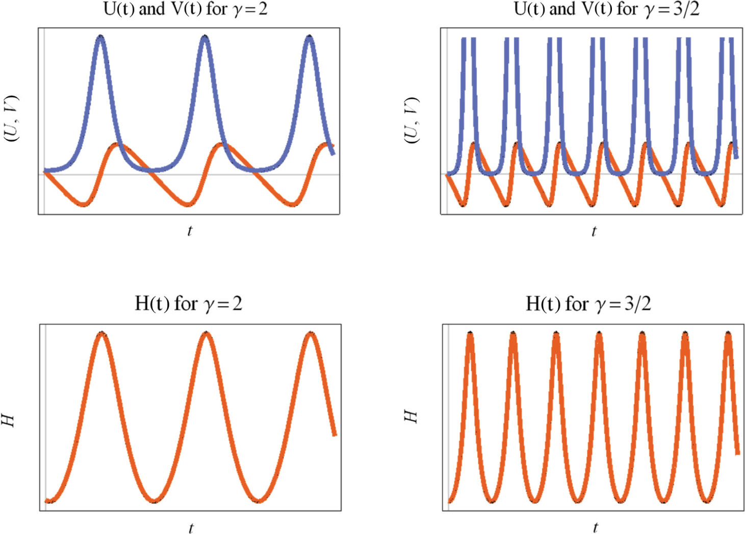
In Figure 1, we present a numerical simulation of the H(ξ) and V(ξ) as they are provided by the differential equation (23). The plots that are presented are for γ = 1.1 and γ = 2. From the figure, we observe a travelling-wave solution for V(ξ) and for the variable H(ξ).

Figure 1:

Qualitative evolution of the functions V(ξ) and H(ξ) provided by the numerical simulation of the nonlinear differential equation (23). The plots are for c = 1 and H₀ = 2 and initial conditions V(0)=0.01, Vξ(0)=−0.2. Left figure is for γ = 1.1, whereas right figure is for γ = 2. We observe that V(ξ) and H(ξ) are periodic functions and have similar behaviour; the different values of γ change only the frequency of the oscillations. However, as we decreased the initial value Vξ(0) in values where c2−(H0−Vξ)−γ−1≃1, the numerical simulation provided singular behaviour for the V(ξ), which corresponds to a shock.

4 Conclusions

In this work, we studied a system of nonlinear PDEs that describe rotating shallow water with the method of Lie symmetries. More specifically, we determine the Lie symmetries for the system (13, 14), and we found that the system of PDEs is invariant under a five-dimensional Lie algebra. The admitted Lie symmetries form the {2A1⊕s 2A1}⊕sA1 Lie algebra in the Morozov–Mubarakzyanov Classification Scheme for the parameter γ > 1 or the 2A1⊕s 3A1 Lie algebra when γ = 1. That difference in the admitted Lie algebra between the two cases γ = 1 and γ ≠ 1 is observable in the application of Lie symmetries and more specifically in the reduction process.

Indeed, for any symmetry vector, we considered the application of the zero-order Lie invariants, and we rewrote the system of PDEs into a system ODEs, which we were able to solve explicitly in all cases by using the Lie symmetry analysis. Another important feature of the Lie symmetries is that we can transform solutions into solutions after the application of the invariant 1PPT.

From the Lie symmetry vectors X₁ − X₅ of the system (13, 14), we determine the generic 1PPT to be

It is important to mention that someone could start the present analysis by studying the original three-dimensional first-order differential equations (1–3). Either in that approach the results of the analysis will not change, except from that the point transformation is defined in the space of variables J={t,x,h,v,u}. In our analysis, we consider to study the point transformations defined in the space of variable I={t,x,h,v}. Now by extending the symmetry vectors obtained in the space I in the (partial-) extension space I′={t,x,h,v,∂v∂t}, the symmetry vectors X1−5 become

where by replacing u=−vt, the Lie point symmetries of the original system (1–3) are found.

We conclude that with the application of Lie symmetries we were able to prove the existence of solutions for the rotating shallow wave system (13, 14). Another important observation is that the reduced differential equations were reduced into well-known first-order ODEs. Finally, we proved the existence of travel-wave and scaling solutions.

References

[1] L. V. Ovsiannikov, Group Analysis of Differential Equations, Academic Press, New York 1982.10.1016/B978-0-12-531680-4.50012-5Suche in Google Scholar
[2] B. K. Harrison, Sigma 1, 001 (2005).10.1504/IJSSCA.2005.008505Suche in Google Scholar
[3] V. A. Baikov, A. V. Gladkov, and R. J. Wiltshire, J. Phys. A: Math. Gen. 31, 7483 (1998).10.1088/0305-4470/31/37/009Suche in Google Scholar
[4] T. G. Mkhize, K. Govinder, S. Moyo, and S. V. Meleshko, Appl. Math. Comput. 301, 25 (2017).10.1016/j.amc.2016.12.019Suche in Google Scholar
[5] A. Paliathanasis and P. G. L. Leach, Int. J. Geom. Meth. Mod. Phys. 13, 1630009 (2016).10.1142/S0219887816300099Suche in Google Scholar
[6] M. C. Nucci and P. G. L. Leach, J. Math. Anal. Appl. 406, 219 (2013).10.1016/j.jmaa.2013.04.050Suche in Google Scholar
[7] M. C. Nucci, J. Nonl. Math. Phys. 20, 451 (2013).10.1080/14029251.2013.855053Suche in Google Scholar
[8] E. Noether, Nachr. d. König. Gesellsch. d. Wiss. zu Göttingen, Math-phys. Klasse, 235 (1918) (translated in English by M. A. Tavel [physics/0503066]).Suche in Google Scholar
[9] N. H. Ibragimov, J. Math. Anal. Appl. 333, 311 (2007).10.1016/j.jmaa.2006.10.078Suche in Google Scholar
[10] W. Sarlet and F. Cantrijin, SIAM Rev. 23, 467 (1981).10.1137/1023098Suche in Google Scholar
[11] P. J. Olver, Applications of Lie Groups to Differential Equations, Springer-Verlag, New York 1993.10.1007/978-1-4612-4350-2Suche in Google Scholar
[12] G. W. Bluman and S. Kumei, Symmetries and Differential Equations, Springer-Verlag, New York 1989.10.1007/978-1-4757-4307-4Suche in Google Scholar
[13] N. H. Ibragimov, CRC Handbook of Lie Group Analysis of Differential Equations, Volume I: Symmetries, Exact Solutions, and Conservation Laws, CRS Press LLC, Florida 2000.Suche in Google Scholar
[14] S. V. Meleshko, Methods for Constructing Exact Solutions of Partial Differential Equations, Springer Science, New York 2005.Suche in Google Scholar
[15] S. V. Meleshko and V. P. Shapeev, J. Nonl. Math. Phys. 18, 195 (2011).10.1142/S1402925111001374Suche in Google Scholar
[16] G. M. Webb and G. P. Zank, J. Math. Phys. A: Math. Theor. 40, 545 (2007).10.1088/1751-8113/40/3/013Suche in Google Scholar
[17] M. C. Nucci and G. Sanchini, Symmetry 7, 1613 (2015).10.3390/sym7031613Suche in Google Scholar
[18] A. Paliathanasis, K. Krishnakumar, K. M. Tamizhmani, and P. G. L. Leach, Mathematics 4, 28 (2016).10.3390/math4020028Suche in Google Scholar
[19] X. Xin, Appl. Math. Lett. 55, 63 (2016).10.1016/j.aml.2015.11.009Suche in Google Scholar
[20] X. Xin, Acta Phys. Sin. 65, 240202 (2016).10.7498/aps.65.240202Suche in Google Scholar
[21] N. Kallinikos and E. Meletlidou, J. Phys. A: Math. Theor. 46, 305202 (2013).10.1088/1751-8113/46/30/305202Suche in Google Scholar
[22] S. Jamal and A. Paliathanasis, J. Geom. Phys. 117, 50 (2017).10.1016/j.geomphys.2017.03.003Suche in Google Scholar
[23] G. M. Webb, J. Phys A: Math. Gen. 23, 3885 (1990).10.1088/0305-4470/23/17/018Suche in Google Scholar
[24] P. G. L. Leach, J. Math. Anal. Appl. 348, 487 (2008).10.1016/j.jmaa.2008.07.018Suche in Google Scholar
[25] M. Tsamparlis and A. Paliathanasis, J. Phys. A: Math. Theor. 44, 175202 (2011).10.1088/1751-8113/44/17/175202Suche in Google Scholar
[26] M. Tsamparlis and A. Paliathanasis, Symmetry (MDPI) 10, 233 (2018).10.3390/sym10070233Suche in Google Scholar
[27] X. Xin, Commun. Theor. Phys. 66, 479 (2016).10.1088/0253-6102/66/5/479Suche in Google Scholar
[28] X. Xin, H. Liu, L. Zhang, and Z. Wang, Appl. Math. Lett. 88, 132 (2019).10.1016/j.aml.2018.08.023Suche in Google Scholar
[29] B. Cheng, P. Qu, and C. Xe, SIAM J. Math. Anal. 50, 2486 (2018).10.1137/17M1130101Suche in Google Scholar
[30] B. Galperin, H. Nakano, H.-P. Huang, and S. Sukoriansky, Geoph. Res. Let. 31, L13303 (2004).10.1029/2004GL019691Suche in Google Scholar
[31] V. Zeitlin, S. B. Medvedev, and R. Plougonven, J. Fluid. Mech. 481, 269 (2003).10.1017/S0022112003003896Suche in Google Scholar
[32] D. A. Randall, Mon. Weather Rev. 122, 1371 (1994).10.1175/1520-0493(1994)122<1371:GAATFD>2.0.CO;2Suche in Google Scholar
[33] M. Senthilvelan and M. Lakshmanan, Int. J. Nonl. Mech. 31, 339 (1996).10.1016/0020-7462(95)00063-1Suche in Google Scholar
[34] S. Szatmari and A. Bihlo, Comm. Nonl. Sci. Num. Sim. 19, 530 (2014).10.1016/j.cnsns.2013.06.030Suche in Google Scholar
[35] A. A. Chesnokov, J. Appl. Mech. Techn. Phys. 49, 737 (2008).10.1007/s10808-008-0092-5Suche in Google Scholar
[36] J.-G. Liu, Z.-F. Zeng, Y. He, and G.-P. Ai, Int. J. Nonl. Sci. Num. Sim. 16, 114 (2013).Suche in Google Scholar
[37] A. A. Chesnokov, Eur. J. Appl. Math. 20, 461 (2009).10.1017/S0956792509990064Suche in Google Scholar
[38] M. Pandey, Int. J. Nonl. Sci. Num. Sim. 16, 93 (2015).10.5455/2320-6012.ijrms20140204Suche in Google Scholar
[39] X. Xin, L. Zhang, Y. Xia, and H. Liu, Appl. Math. Lett. 94, 112 (2019).10.1016/j.aml.2019.02.028Suche in Google Scholar
[40] V. V. Morozov, Izv. Vyssh. Uchebn. Zaved. Mat. 5, 161 (1958).Suche in Google Scholar
[41] G. M. Mubarakzyanov, Izv. Vyssh. Uchebn. Zaved. Mat. 32, 114 (1963).Suche in Google Scholar
[42] G. M. Mubarakzyanov, Izv. Vyssh. Uchebn. Zaved. Mat. 34, 99 (1963).Suche in Google Scholar
[43] G. M. Mubarakzyanov, Izv. Vyssh. Uchebn. Zaved. Mat. 35, 104 (1963).Suche in Google Scholar
[44] P. J. Olver, Applications of Lie Groups to Differential Equations, Second Edition, Springer-Verlag, New York 1993.10.1007/978-1-4612-4350-2Suche in Google Scholar
[45] X. Hu, Y. Li and Y. Chen, J. Math. Phys. 56, 053504 (2015).10.1063/1.4921229Suche in Google Scholar
[46] V. Ermakov, Univ. Izv. Kiev Ser. III, 9, 1 (1880) (The English version, translated by A. O. Harin, can be found in Applicable analysis and Discrete Mathematics).Suche in Google Scholar
[47] E. Pinney, P. Am. Math. Soc. 1, 681 (1950).10.1090/S0002-9939-1950-0037979-4Suche in Google Scholar
©2019 Walter de Gruyter GmbH, Berlin/Boston
Artikel in diesem Heft
- Frontmatter
- Solid State Physics & Materials Science
- Electronic and Optical Properties of Cubic Perovskites CsPbCl3−yIy (y = 0, 1, 2, 3)
- Effect of Indium Doping on Optical Parameter Properties of Sol–Gel-Derived ZnO Thin Films
- Electrical Conductivity of Zirconium Tetrachloride Solutions in Molten Sodium, Potassium and Cesium Chlorides
- Hydrogen Sulfide Gas Sensor Based on Copper/Graphene Oxide Composite Film-Coated Tapered Single-Mode Fibre Interferometer
- Dynamical Systems & Nonlinear Phenomena
- Detecting the Flow Pattern Transition in the Gas-Liquid Two-Phase Flow Using Multivariate Multi-Scale Entropy Analysis
- Rapid Communication
- Simplistic Synthesis and Enhanced Photocatalytic Performance of Spherical ZnO Nanoparticles Prepared from Arabinose Solution
- The Deflection of Rotating Composite Tapered Beams with an Elastically Restrained Root in Hygrothermal Environment
- Effect of Dust Ion Collision on Dust Ion Acoustic Solitary Waves for Nonextensive Plasmas in the Framework of Damped Korteweg–de Vries–Burgers Equation
- Hydrodynamics
- Lie Symmetries and Similarity Solutions for Rotating Shallow Water
- A Note on the Significance of Quartic Autocatalysis Chemical Reaction on the Motion of Air Conveying Dust Particles