Detecting the Flow Pattern Transition in the Gas-Liquid Two-Phase Flow Using Multivariate Multi-Scale Entropy Analysis
-
Yudong Liu


Abstract
Due to the complex flow structure and non-uniform phase distribution in the vertical upward gas-liquid two-phase flow, an eight-electrode rotating electric field conductance sensor is used to obtain multi-channel conductance signals. The flow patterns of the vertical upward gas-liquid two-phase flow are classified according to the images obtained from a high-speed camera. Then, we employ the multivariate weighted multi-scale permutation entropy (MWMPE) to detect the instability of flow pattern transition in the gas-liquid two-phase flow. Afterwards, we compare the results of the MWMPE with those of the single-channel weighted multi-scale permutation entropy (SCWMPE) and multivariate multi-scale sample entropy (MMSE). The comparison results indicate that, compared with the SCWMPE and MMSE, the MWMPE has superior performance in terms of the high-resolution presentation of flow instability in the gas-liquid two-phase flow. Finally, we extract the mean value of the MWMPE in whole scales and the entropy rate of the MWMPE in the small scales. The results indicate that the normalized mean value and normalized entropy rate of MWMPE are very sensitive to the transitions of flow patterns, thus allowing the detection of the instability of flow pattern transition.
1 Introduction
The gas-liquid two-phase flow widely exists in industrial production processes, such as petroleum exploitation, nuclear reactor, chemical industry, metallurgy, etc. Due to the complex flow structure and non-uniform phase distribution in the gas-liquid two-phase flow as well as the severe slippage effect between the light phase and the heavy phase, the gas-liquid two-phase flow shows highly instable dynamic characteristics. Investigating the unstable dynamic characteristics of the gas-liquid two-phase flow pattern transition is of great significance to understanding the flow mechanism of the gas-liquid two-phase flow, the sensor design and its geometry optimization and the modelling of flow measurement.
The studies on the flow characteristics of multiphase flow mainly include the direct and indirect methods. The direct method intuitively obtains the flow patterns of the multiphase flow based on flow visualization, including the visual inspection method and the high-speed camera method. The indirect method characterizes the flow characteristics of the multiphase flow by analyzing its fluctuation signals through statistical analysis, time-frequency spectrum analysis and nonlinear analysis. In the aspect of statistical analysis methods, Hubbard and Dukler [1] divided the horizontal gas-liquid two-phase flow patterns into separated flow, dispersed flow and intermittent flow based on the power spectrum density distribution (PSD) method of the wall static pressure fluctuation signals. Jones Jr. and Zuber [2] obtained the local void fraction signals of the gas-liquid two-phase flow in a square pipeline based on the X-ray method, and applied the probability density function (PDF) method to identify three flow patterns, including bubble flow, slug flow and annular flow, in the gas-liquid two-phase flow. Later, Vince and Lahey [3] used the X-ray system, applied the PDF and PSD methods simultaneously and finally obtained similar results as those of Jones and Zuber [2]. In the aspect of time-frequency spectrum analysis methods, the time-frequency spectrum signals analysis method, such as wavelet transform [4], [5], [6], Hilbert–Huang transform (HHT) [7], [8] and adaptive optimal kernel (AOK) [9], [10], [11], have been widely used in the gas-liquid two-phase flow analysis.
Entropy, as a measure of system complexity, plays a significant role in the analysis of nonlinear dynamic characteristics. The approximate entropy algorithm, proposed by Pincus [12] to analyze time series irregularities, is widely used in the field of biomedical signals processing [13], [14]. However, the approximate entropy is not suitable for analyzing time series with short length and noise. Richman and Moorman [15] proposed the sample entropy algorithm based on the approximate entropy algorithm. Considering that the complex systems are susceptible to interference of environmental noise, Bandt and Pompe [16] proposed the permutation entropy algorithm. In order to compensate for permutation entropy algorithm’s defect (i.e. losing the original time series amplitude information in the analysis process), Fadlallah et al. [17] proposed the weighted permutation entropy algorithm to explore the amplitude information in the time series and improve the robustness and anti-noise ability of permutation entropy algorithm. Based on the multi-scale sample entropy coarse-graining algorithm proposed by Costa et al. [18], Zheng et al. [19] applied multi-scale sample entropy (MSE) to analyze the conductance fluctuation signals of the gas-liquid two-phase flow, and proved that multi-scale sample entropy can reveal the dynamic complex characteristics of bubble flow, churn flow and slug flow at different scales. In recent years, substantial progress has been made in the field of multivariate multi-scale entropy algorithm analysis [20], [21]. In particular, Yin et al. [22] proposed the multivariate weighted multi-scale permutation entropy (MWMPE) and pointed out its advantages in terms of high resolution and robustness to noisy signals in multivariate time series analysis.
Our research group has compared the anti-noise performance of four typical multivariate multi-scale entropy algorithms, including multivariate weighted multi-scale permutation entropy (MWMPE), multivariate multi-scale permutation entropy (MMPE), multivariate multi-scale sample entropy (MMSE) as well as multivariate multi-scale approximate entropy (MMAE), and the results indicate that MWMPE is advantageous in revealing the flow instability of vertical upward oil-water two-phase flow [23]. To further characterize the instability of the flow pattern transition in the vertical upward gas-liquid two-phase flow, an eight-electrode rotating electric field conductance sensor is utilized. This is done in order to obtain the multi-channel conductance signals of the gas-liquid two-phase flow in different directions of the pipe cross-section. A comparison of the results of the MWMPE with those of the SCWMPE and MMSE indicate that the MWMPE has the advantage of high resolution presentation in revealing flow instability in the gas-liquid two-phase flow. Finally, we extract the mean value of the MWMPE in whole scales and the entropy rate of MWMPE in small scales. The flow instability of the flow pattern transition is also detected in the joint distribution of normalized mean value and normalized entropy rate in the MWMPE.
2 Methodology
2.1 Multivariate Coarse-Graining Algorithm
Given the multivariate time series, we employ the multi-scale coarse-graining algorithm proposed by Costa et al. [18] to implement the multivariate multi-scale calculation. The m-dimensional time series can be expressed as
where s refers to the scale factor. The length of time series of the coarse-graining m-dimensional time series in each dimension is equal to the length of primitive time series N divided by scale factor s in the corresponding dimension.
2.2 Multivariate Multi-Scale Weighted Permutation Entropy Algorithm
Given the m-dimensional primitive time series
By sorting the whole components of
If there exist components with an identical value in
For a phase space with an embedding dimension equal to d, the total number of permutation is d!. We define the number of occurrences of the jth permutation as Nj, where 1 ≤ j ≤ d!. Moreover, we, respectively define
The weighted probability
For the m-dimensional primitive time series,
Then the MWMPE can be expressed with the following form of Shannon entropy:
Based on the same principle, the definition of the SCWMPE can be obtained as follows:
2.3 Multivariate Multi-Scale Sample Entropy Algorithm
Given the m-dimensional primitive time series
where
Next, we set a threshold r, counting the occurrence number Qi that satisfies
where Bd(r) is defined as the probability that any two phase-space vectors are close for embedding dimensions of d. Based on the same principle, we increase the embedding dimension of the multivariate series phase space vector from d to d + 1, thus obtaining the following formula:
The expression of MMSE is given as follows:
3 Experimental Facility and Signal Acquisition
3.1 Experimental Facility
The experiment of the vertical upward gas-liquid two-phase flow was implemented in the lab of multiphase flow sensor system and fluid flow in Tianjin University. The schematic diagram of the experimental facility is shown in Figure 1. The experimental pipe is made up of acrylic material with an inner diameter of 20 mm and a length of 2820 mm. The experimental flow media are air and tap water. The industrial peristaltic pump is utilized to transport and control the flux of the liquid phase. The air compressor is utilized to generate the gas phase and the flux of gas phase is metered by the float flowmeter. The gas and liquid phase with a certain ratio are uniformly mixed in the mixer at the inlet and then injected into the experimental pipe. During the experiment, the gas superficial velocity Usg is fixed at first, then we gradually change the liquid superficial velocity Usl to carry out the experiment. After all the liquid superficial velocities are finished, we change the gas superficial velocity to the next value, and then the experiments are repeated in the above way. In the experiment, the gas superficial velocity Usg varies from 0.0553 m/s to 0.6624 m/s, and the liquid superficial velocity Usl varies from 0.0368 m/s to 1.1776 m/s. The flow conditions are shown in Table 1.
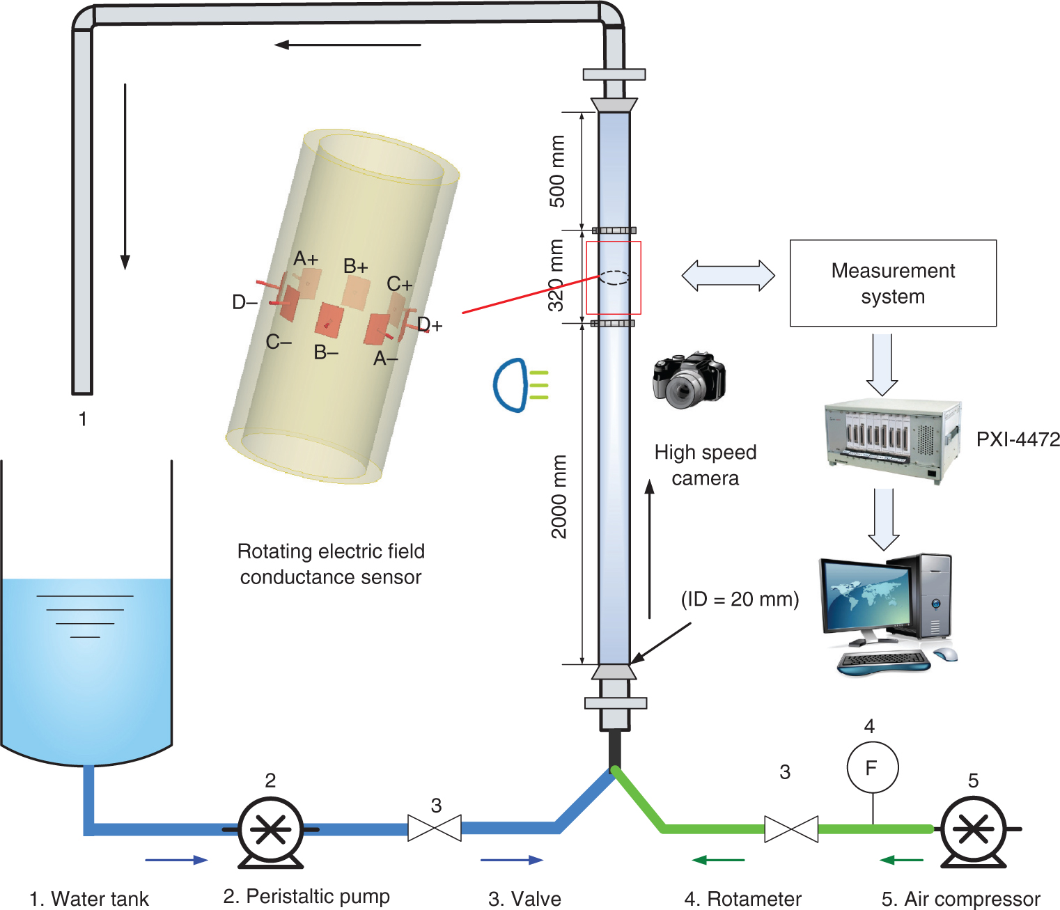
The schematic diagram of THE vertical upward gas-liquid two-phase flow experimental facility.
The flow conditions of the gas-liquid two-phase flow in the vertical upward pipe.
| Usg (m/s) | Usl (m/s) | Flow pattern | Usg (m/s) | Usl (m/s) | Flow pattern | ||
|---|---|---|---|---|---|---|---|
| 1 | 0.0552 | 0.0368 | Slug flow | 29 | 0.2944 | 0.5888 | Slug flow |
| 2 | 0.0552 | 0.0736 | Slug flow | 30 | 0.2944 | 0.8832 | Churn flow |
| 3 | 0.0552 | 0.1472 | Slug flow | 31 | 0.2944 | 1.0304 | Churn-bubble flow |
| 4 | 0.0552 | 0.2944 | Slug flow | 32 | 0.2944 | 1.1776 | Bubble flow |
| 5 | 0.0552 | 0.5888 | Slug flow | 33 | 0.4416 | 0.0368 | Slug flow |
| 6 | 0.0552 | 0.8832 | Bubble flow | 34 | 0.4416 | 0.0736 | Slug flow |
| 7 | 0.0552 | 1.0304 | Bubble flow | 35 | 0.4416 | 0.1472 | Slug flow |
| 8 | 0.0552 | 1.1776 | Bubble flow | 36 | 0.4416 | 0.2944 | Slug flow |
| 9 | 0.0736 | 0.0368 | Slug flow | 37 | 0.4416 | 0.5888 | Slug flow |
| 10 | 0.0736 | 0.0736 | Slug flow | 38 | 0.4416 | 0.8832 | Churn flow |
| 11 | 0.0736 | 0.1472 | Slug flow | 39 | 0.4416 | 1.0304 | Churn flow |
| 12 | 0.0736 | 0.2944 | Slug flow | 40 | 0.4416 | 1.1776 | Bubble flow |
| 13 | 0.0736 | 0.5888 | Slug flow | 41 | 0.5888 | 0.0368 | Slug flow |
| 14 | 0.0736 | 0.8832 | Bubble flow | 42 | 0.5888 | 0.0736 | Slug flow |
| 15 | 0.0736 | 1.0304 | Bubble flow | 43 | 0.5888 | 0.1472 | Slug flow |
| 16 | 0.0736 | 1.1776 | Bubble flow | 44 | 0.5888 | 0.2944 | Slug flow |
| 17 | 0.1472 | 0.0368 | Slug flow | 45 | 0.5888 | 0.5888 | Slug flow |
| 18 | 0.1472 | 0.0736 | Slug flow | 46 | 0.5888 | 0.8832 | Churn flow |
| 19 | 0.1472 | 0.1472 | Slug flow | 47 | 0.5888 | 1.0304 | Churn flow |
| 20 | 0.1472 | 0.2944 | Slug flow | 48 | 0.5888 | 1.1776 | Churn flow |
| 21 | 0.1472 | 0.5888 | Slug flow | 49 | 0.6624 | 0.0368 | Slug flow |
| 22 | 0.1472 | 0.8832 | Churn-bubble flow | 50 | 0.6624 | 0.0736 | Slug flow |
| 23 | 0.1472 | 1.0304 | Bubble flow | 51 | 0.6624 | 0.1472 | Slug flow |
| 24 | 0.1472 | 1.1776 | Bubble flow | 52 | 0.6624 | 0.2944 | Slug flow |
| 25 | 0.2944 | 0.0368 | Slug flow | 53 | 0.6624 | 0.5888 | Slug flow |
| 26 | 0.2944 | 0.0736 | Slug flow | 54 | 0.6624 | 0.8832 | Churn flow |
| 27 | 0.2944 | 0.1472 | Slug flow | 55 | 0.6624 | 1.0304 | Churn flow |
| 28 | 0.2944 | 0.2944 | Slug flow | 56 | 0.6624 | 1.1776 | Churn flow |
In this study, an eight-electrode rotating electric field conductance sensor [25] is used to capture the flow structure information of the gas-liquid two-phase flow from different directions of the pipe cross section. As stated in the descriptions in [25], the eight-electrode rotating electric field conductance sensor presents the high sensitivity and homogeneous sensitivity distribution under optimal geometric parameters, which means that the sensor can possess high resolution in water holdup variation caused by flow structural change. Moreover, the output of the sensor is a linear function of the conductivity; therefore, this sensor can well acquire flow structure information from different directions of the pipe cross-section with high resolution. As shown in Figure 1, the sensor consists of eight stainless steel electrodes that are flush-mounted on the inner wall of a 20 mm inner diameter pipe. In order to acquire the fully developed gas-liquid two-phase flow information, the eight-electrode rotating electric field conductance sensor is installed in the testing pipe with a distance of 2000 mm from the pipe inlet. The working principle of the eight-electrode rotating electric field conductance sensor is as follows: sinusoidal excitation signals with peak-to-peak value of 10 V, frequency of 20 kHz and fixed phase are applied to the electrodes (A+, B+, C+, D+, A−, B−, C−, D−) simultaneously, as shown in Figure 1, and the phase difference between adjacent excitation signals is 45°. Then, a rotating electric field in the sensor volume is obtained. By modulating the output voltage between A+ and A−, B+ and B−, C+ and C− and D+ and D−, the corresponding A, B, C and D four-channel signals, which can reflect the flow structure information of the gas-liquid two-phase flow, can be obtained. The four-channel signals are sampled by NI PXI-4472 synchronous acquisition card. The sampling time and sampling frequency are 30 s and 2 kHz, respectively.
The flow patterns can be directly observed and determined by the images of the gas-liquid two-phase flow captured by a high-speed camera. As shown in Figure 2, there are four typical flow patterns in the two-phase flow, namely, slug flow, churn flow, bubble flow and churn-bubble transitional flow. As shown in Figure 2a, the slug flow is mainly composed of the Taylor bubble, falling liquid film and liquid slug. The Taylor bubbles occupy most of the pipe section. The falling liquid films with a small number of gas bubbles exist between the pipe wall and the Taylor bubble. The liquid slugs contain a large number of gas bubbles with different sizes. The Taylor bubbles and liquid slugs appear as quasi-periodic alternating motion. The images of churn flow are shown in Figure 2b. As can be seen, the churn flow is characterized by the distortion of the interface between the gas phase and the liquid phase and the random flow phenomenon in which the gas phase and the liquid phase are oscillated up and down in the pipe. In the bubble flow as presented in Figure 2c, gas bubbles with different sizes are non-uniformly distributed in the liquid phase and their motions have strong randomness. In the churn-bubble transitional flow shown in Figure 2d, the distortion of the interface between the gas phase and the liquid phase as well as the non-uniform distribution of bubbles with different sizes in the liquid phase exist simultaneously.

The four typical flow pattern images captured by THE high-speed camera. (a) Slug flow (Usg = 0.0553 m/s, Usl = 0.0736 m/s). (b) Churn flow (Usg = 0.4416 m/s, Usl = 0.8832 m/s). (c) Bubble flow (Usg = 0.0736 m/s, Usl = 1.1776 m/s). (d) Churn-bubble transitional flow (Usg = 0.1472 m/s, Usl = 0.8832 m/s).
3.2 Fluctuating Signals of the Rotating Electric Field Conductance Sensor
The four-channel fluctuating signals of the typical slug flow are shown in Figure 3a. As can be seen, the slug flow signals have a large fluctuation range. The peak value of the voltage signal can reach about 3.2 V, while the lowest value is about 0.8 V. When the liquid slugs pass through the conductance sensor, the conductance between the electrodes increases, then the fluctuating signals show a high voltage. Moreover, as the Taylor bubbles pass through the conductance sensor, they occupy most of the pipe section, resulting in a decrease of conductance between the electrodes, with the fluctuating signals showing a low voltage. The high and low voltages appear alternately, corresponding to the behavior of Taylor bubbles and liquid slugs appearing as quasi-periodic alternating motion.

The rotating electric field conductance sensor signals. (a) Slug flow; (b) churn flow; (c) bubble flow; (d) churn-bubble transitional flow.
The four-channel fluctuating signals of the typical churn flow are shown in Figure 3b. The fluctuating signals have a short duration of high voltage and low voltage and the fluctuation is random. Due to the increase of the gas and liquid superficial velocity, the large gas slug is crushed into a number of gas blocks with different sizes. The gas blocks and the liquid phases appear alternately and randomly, exhibiting disorderly motion characteristics.
The four-channel fluctuating signals of a typical bubble flow are shown in Figure 3c. The fluctuating range of measurement signals is in the range of 2.4–3.2 V. The highly intense fluctuation is consistent with the flow characteristics of the irregular random motion of a large number of bubbles with different sizes in the bubble flow.
The four-channel fluctuating signals of a typical churn-bubble transitional flow are shown in Figure 3d. The measurement signals appear in the form of irregular fluctuation with a small amplitude, thus conforming to the flow characteristics of the bubble flow. In addition, some signal fluctuations with large interval and large amplitude are consistent with the flow characteristics of the churn flow. Based on the above flow characteristics, the flow pattern conforms to the churn-bubble transitional flow pattern under this flow condition.
4 Flow Instability Analysis of the Gas-Liquid Two-Phase Flow
4.1 Multivariate Weighted Multi-Scale Permutation Entropy Analysis
In this section, the MWMPE is employed to analyze the gas-liquid two-phase flow fluctuation signals measured by the eight-electrode rotating electric field conductance sensor. First, we set the parameters during the MWMPE calculation process. The maximum coarse-graining scale is set to 20, which is sufficient for multi-scale analysis. The signal sequence length is set to 10,000, which can fully reflect the flow characteristics of the gas-liquid two-phase flow. The value of the embedding dimension d for all flow conditions is set to 6 using the method of the false nearest neighbors (FNN) [26]. According to descriptions in [16], the authors of the permutation entropy recommend setting the embedding dimension to 3, 4, …, 7, with the time delay τ assigned as 1. Hence, we set the embedding dimension d and the time delay τ as 6 and 1 for all flow conditions, respectively.
In order to further verify the feasibility of the selected embedding dimension d and time delay τ, we explore the calculation results of the MWMPE with different embedding dimensions and different delay times, as shown in Figure 4. We set the time delay τ as 1 and then change the embedding dimension from 3 to 7 to observe the sensibility of the MWMPE in one flow condition. The calculation results of the MWMPE using different d values are shown in Figure 4a. Under the same flow condition, with the increase of d, the calculation results of the MWMPE present an increasing trend. We find that when d is 6, the calculation results of the MWMPE present better increasing trend in the whole scales than other calculation results with different d values. Then, we set the embedding dimension as 6 and change the time delay from 1 to 5 to observe the sensibility of MWMPE in the same flow condition. The calculation results of the MWMPE in different τ values are shown in Figure 4b. Under the same flow condition, with the increase of τ, the calculation results of the MWMPE also present an increasing trend. We find that, when τ is 1, the calculation results of the MWMPE present better increasing trend in the whole scales than other calculation results with different τ values. Setting the embedding dimension as 6 and the time delay τ as 1 can effectively reflect the difference of entropy values at different scales.

The calculation results of the MWMPE in different values of d and τ. (a) The calculation results of the MWMPE in different values of d. (b) The calculation results of the MWMPE in different values of τ.
Figure 5 presents the calculation results of the MWMPE for the measurement signals from the eight-electrode rotating electric field conductance sensor under different flow conditions. As shown in Figure 5, the MWMPE values in four typical flow patterns have significant differences within the whole scales. The MWMPE values in bubble flow remained the highest, whereas the MWMPE values in the slug flow are the lowest. The MWMPE values in the churn flow and churn-bubble transitional flow are between the slug flow and bubble flow. Moreover, the churn-bubble transitional flow has the higher MWMPE values than churn flow. It should be noted that the increase of entropy values in small scales, which is defined as the growth rate of the MWMPE, varies significantly in different flow patterns. The growth rate of the MWMPE in the bubble flow is the highest, whereas the growth rate in the churn-bubble transitional flow is lower than that in the bubble flow. The churn flow presents a lower growth rate than the churn-bubble transitional flow. The growth rate of the MWMPE in the slug flow is the lowest. The above calculation results are related to the flow characteristics of the corresponding flow patterns.
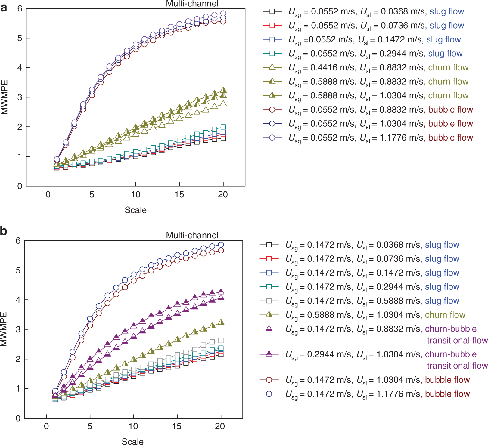
The calculation results of the MWMPE in the gas-liquid two-phase flow. (a) The calculation results of the MWMPE in slug flow, churn flow and bubble flow. (b) The calculation results of the MWMPE in slug flow, churn flow, churn-bubble transitional flow and bubble flow.
For the slug flow, the Taylor bubbles and the liquid slugs alternately rise and pass through the conductance sensor with a certain quasi-periodic movement characteristic; therefore, the flow characteristic of the slug flow are relatively stable, and the MWMPE values in the slug flow are low in the whole scales. As the increasing liquid superficial velocity enhances the overall turbulent energy, the Taylor bubbles are crushed into bubbles with different sizes and are randomly distributed in the liquid phase; the flow pattern then evolves to the bubble flow with the highest MWMPE values in the whole scales. When the gas superficial velocity and liquid superficial velocity both increase, the Taylor bubbles in the slug flow are broken into a number of irregular gas blocks with a turbulent movement, and the flow pattern gradually evolves to churn flow. The instability of the churn flow is higher than the slug flow, which presents a quasi-periodic motion behavior; at the same time, it is lower than the bubble flow with random motion behavior. Therefore, the MWMPE of the churn flow is between the slug flow and the bubble flow in the whole scales. The churn-bubble transitional flow forms in the process of churn flow evolving into bubble flow; therefore, the MWMPE of the churn-bubble transitional flow is higher than the churn flow and lower than the bubble flow. Moreover, under one flow pattern condition, with the increase of the total mixture velocity, the turbulent energy of the gas-liquid two-phase flow is enhanced, which then increases the flow instability of the gas-liquid two-phase flow. Therefore, the MWMPE in the whole scales shows an increasing trend. Moreover, the MWMPE can effectively reveal the flow instability of the gas-liquid two-phase flow during the flow pattern transition.
4.2 Single-Channel Weighted Multi-Scale Permutation Entropy Analysis
In order to assess the advantages of the MWMPE in the flow instability of the gas-liquid two-phase flow, in this section, the SCWMPE is employed to analyze the gas-liquid two-phase flow fluctuation signals measured by the eight-electrode rotating electric field conductance sensor. As shown in Figure 6, the calculation results of SCWMPE for the measurement fluctuating signals of channel A and channel C from the eight-electrode rotating electric field conductance sensor under different typical flow conditions are given.

The calculation results of the SCWMPE in the gas-liquid two-phase flow. (a) The calculation results of the SCWMPE in channel A. (b) The calculation results of the SCWMPE in channel C. (c) The calculation results of the SCWMPE in channel A. (d) The calculation results of the SCWMPE in channel C.
Figure 6a,b are the calculation results of the SCWMPE in channel A and channel C, respectively, which can be compared with the calculation results of the MWMPE in Figure 5a. As shown in Figure 6a,b, the calculation results of the SCWMPE can reveal the instability of different flow patterns. However, its resolution in uncovering the instability of flow condition variation under the same flow pattern is limited, especially in the bubble flow and slug flow in large scales. Furthermore, the MWMPE values increase steadily with the increase of scales. However, the SCWMPE values are fluctuant in large scales. Similarly, the calculation results of SCWMPE in Figure 6c,d can be compared with the calculation results of MWMPE in Figure 5b. It can be found that the calculation results of SCWMPE in channel A shown in Figure 6c is similar to the calculation results of MWMPE in Figure 5b. However, the calculation results of SCWMPE in channel C present poor capacity in uncovering the instability of different flow patterns under different flow conditions. Single-channel signals only reflect the flow characteristics of the local measured section, so the weighted multi-scale permutation entropy based on the single-channel signals cannot accurately reflect the flow instability of the gas-liquid two-phase flow in detail. In summary, the MWMPE show its superiority in revealing the flow instability of gas-liquid two-phase flow compared with the SCWMPE.
4.3 Multivariate Multi-Scale Sample Entropy Analysis
In light of the descriptions in [23], the MWMPE demonstrated anti-noise performance in relation to some typical time series and its superior ability to reveal the flow instability of the vertical upward oil-water two-phase flow. In addition, we find that the MMSE also presents satisfactory performance. Hence, we choose the MMSE analysis as a comparator to the MWMPE. Figure 7a,b illustrate the calculation results of the MMSE in typical flow pattern conditions. It can be seen from Figure 7a that the MMSE analysis can identify three typical flow patterns through the entropy values, but the MMSE values are fluctuant in large scales, especially in the bubble flow and churn flow. This is because the multi-scale sample entropy has an inherent defect in that the multi-scale sample entropy may yield an inaccurate estimation of entropy as the coarse-graining procedure reduces considerably the length of a time series in large scales [27]. The resolution of the MMSE in uncovering the instability of the flow condition variation is limited in the bubble flow, slug flow and transitional flow. In addition, it can also be seen from Figure 7b that the MMSE cannot identify churn flow and churn-bubble transitional flow. Therefore, compared with the MMSE, the MWMPE analysis presents better performance against the flow instability of the vertical upward gas-liquid two-phase flow.

The calculation results of the MMSE in the gas-liquid two-phase flow. (a) The calculation results of the MMSE in the slug flow, churn flow and bubble flow. (b) The calculation results of the MMSE in the slug flow, churn flow, churn-bubble transitional flow and bubble flow.
4.4 Joint Distribution of the Normalized Mean Value and Normalized Entropy Rate in the MWMPE
To further characterize the flow instability of the flow pattern transition in the gas-liquid two-phase flow, we extract the mean value of MWMPE in whole scales and the entropy rate of MWMPE in small scales under the whole flow conditions. The mean value of the MWMPE is determined by calculating the MWMPE values in the whole scales. As for the determination of the entropy rate, we define the slope obtained by linearly fitting the MWMPE calculation results in the scale range of 1–5 as the entropy rate. As stated in Section 4.1, the MWMPE values present a high increasing rate with the increase of scale in small scales; moreover, the increasing rates vary among different flow patterns. Therefore, the MWMPE range in the small scales can be considered as a sensitive area for the gas-liquid two-phase flow pattern transition. Thus, we carry out the normalization process in the mean value and entropy rate of the MWMPE using the following formula and then build the graph of joint distribution as shown in Figure 8.

The joint distribution of the normalized mean value and normalized entropy rate in the MWMPE.
In the formula above, z is the mean value or the entropy rate of the MWMPE, and z∗ is the normalized mean value (NM) or the normalized entropy rate (NR) of the MWMPE. As shown in Figure 8, the normalized mean value and normalized entropy rate of the slug flow are the smallest, indicating that the flow characteristic is the most stable. In comparison, the normalized mean value and normalized entropy rate of the bubble flow are the highest, indicating that the flow instability is the most obvious. The normalized mean value and normalized entropy rate of the churn flow and churn-bubble transitional flow are between the slug flow and bubble flow, which are consistent with their dynamic flow instability.
The joint distribution of the normalized mean value and normalized entropy rate in the MWMPE can satisfactorily indicate flow instability boundaries between different flow patterns. As shown in Figure 8, the five boundaries are NM = 0.21, NM = 0.38, NM = 0.72, NR = 0.25 and NR = 0.67, respectively. The flow instability of the bubble flow is maximal and it mainly lies in NM ≥ 0.72 and NR ≥ 0.67. The main region of the churn-bubble transitional flow is 0.38 ≤ NM ≤ 0.72, 0.25 ≤ NR ≤ 0.67, churn flow is 0.21 ≤ NM ≤ 0.38 and slug flow is NM ≤ 0.21. In conclusion, the MWMPE can satisfactorily detect flow pattern transition in the gas-liquid two-phase flow using the multivariate multi-scale entropy analysis.
5 Conclusion
In the present study, we employ an eight-electrode rotating electric field conductance sensor to obtain the multi-channel conductance signals of different flow patterns from different directions of the pipe cross-section. The flow patterns of the gas-liquid two-phase flow are classified based on the images obtained from a high-speed camera. Then, the MWMPE, MMSE and SCWMPE are applied to reveal the flow instability of the two-phase flow and their performances are evaluated. Afterwards, we characterize the flow instability of the gas-liquid two-phase flow pattern transition in the joint distribution of the normalized mean value and normalized entropy rate in the MWMPE. The conclusions can be summarized as follows:
The Taylor bubbles and liquid slugs in the slug flow appear in a quasi-periodic alternating motion; therefore, the MWMPE values are the lowest, indicating the lowest flow instability. For bubble flow, a large number of bubbles with different sizes are non-uniformly distributes in the liquid phase and the movement of bubbles is extremely random; thus; the MWMPE values are the highest. The MWMPE values in the churn flow are larger than those in the slug flow due to the chaotic and disordered flow structure, though it is smaller than that of the bubble flow. As the churn-bubble transitional flow appearing in the process of churn flow evolve to bubble flow, its MWMPE values are between the churn flow and bubble flow.
By comparing the results of the SCWMPE and the MMSE with the results of the MWMPE, the superiorities of the MWMPE in revealing the flow instability of flow pattern transition in the gas-liquid two-phase flow is verified. Moreover, through extracting the mean value of the MWMPE in whole scales and the entropy rate of MWMPE in the small scales, the joint distribution is built and the flow instability of the flow pattern transition in the gas-liquid two-phase flow can be effectively characterized using the joint distribution of the normalized mean value and the normalized entropy rate in the MWMPE.
Funding source: National Natural Science Foundation of China
Award Identifier / Grant number: 51527805
Award Identifier / Grant number: 11572220
Funding statement: This study was supported by the National Natural Science Foundation of China (Funder Id: http://dx.doi.org/10.13039/501100001809, Grant Nos. 51527805 and 11572220).
References
[1] M. G. Hubbard and A. E. Dukler, The Characterization of Flow Regimes for Horizontal Two-Phase, Proceeding of 1996 Heat Transfer and Fluid Mechanics Institute, Stanford University Press 1996, p. 100.Search in Google Scholar
[2] O. C. Jones Jr. and N. Zuber, Int. J. Multiph. Flow 2, 273 (1975).10.1016/0301-9322(75)90015-4Search in Google Scholar
[3] M. A. Vince and R. T. Lahey Jr., Int. J. Multiph. Flow 8, 93 (1982).10.1016/0301-9322(82)90012-XSearch in Google Scholar
[4] B. R. Bakshi, H. Zhong, P. Jiang, and L. S. Fan, Chem. Eng. Res. Des. 73, 608 (1995).Search in Google Scholar
[5] T. Elperin and M. Klochko, Exp. Fluids 32, 674 (2002).10.1007/s00348-002-0415-xSearch in Google Scholar
[6] V. T. Nguyen, J. E. Dong, and C. H. Song, Int. J. Multiph. Flow 36, 755 (2010).10.1016/j.ijmultiphaseflow.2010.04.007Search in Google Scholar
[7] Z. K. Peng, P. W. Tse, and F. L. Chu, Mech. Syst. Signal Process. 19, 974 (2005).10.1016/j.ymssp.2004.01.006Search in Google Scholar
[8] H. Ding, Z. Huang, Z. Song, and Y. Yan, Flow. Meas. Instrum. 18, 37 (2007).10.1016/j.flowmeasinst.2006.12.004Search in Google Scholar
[9] B. Sun, E. Wang, D. Yang, Y. Ding, H. Z. Bai, et al., Chin. J. Chem. Eng. 19, 243 (2011).10.1016/S1004-9541(11)60161-4Search in Google Scholar
[10] B. Sun, E. Wang, and Y. J. Zheng, Acta Phys. Sin. 60, 381 (2011).Search in Google Scholar
[11] M. Du, N. D. Jin, Z. K. Gao, and B. Sun, Chem. Eng. Sci. 82, 144 (2012).10.1016/j.ces.2012.07.028Search in Google Scholar
[12] S. M. Pincus, Proc. Natl. Acad. Sci. U.S.A. 88, 2297 (1991).10.1073/pnas.88.6.2297Search in Google Scholar PubMed PubMed Central
[13] S. M. Pincus and R. R. Viscarello, Obstet. Gynecol. 79, 249 (1992).Search in Google Scholar
[14] L. A. Fleisher, S. M. Pincus, and S. H. Rosenbaum, Anesthesiology 78, 683 (1993).10.1097/00000542-199304000-00011Search in Google Scholar PubMed
[15] J. S. Richman and J. R. Moorman, Am. J. Physiol. Heart Circ. Physiol. 278, 2039 (2000).10.1152/ajpheart.2000.278.6.H2039Search in Google Scholar
[16] C. Bandt and B. Pompe, Phys. Rev. Lett. 88, 174102 (2002).10.1103/PhysRevLett.88.174102Search in Google Scholar
[17] B. Fadlallah, B. Chen, A. Keil, and J. Príncipe, Phys. Rev. E. 87, 022911 (2013).10.1103/PhysRevE.87.022911Search in Google Scholar
[18] M. Costa, A. L. Goldberger, and C. K. Peng, Phys. Rev. Lett. 89, 068102 (2002).10.1103/PhysRevLett.89.068102Search in Google Scholar
[19] G. B. Zheng and N. D. Jin, Acta Phys. Sin. 58, 4485 (2009).10.7498/aps.58.4485Search in Google Scholar
[20] M. U. Ahmed and D. P. Mandic, Phys. Rev. E 84, 061918 (2011).10.1103/PhysRevE.84.061918Search in Google Scholar
[21] Z. K. Gao, Y. X. Yang, L. S. Zhai, M. S. Ding and N. D. Jin, Chem. Eng. J. 291, 74 (2016).10.1016/j.cej.2016.01.039Search in Google Scholar
[22] Y. Yin and P. J. Shang, Nonlinear Dyn. 88, 1707 (2017).10.1007/s11071-017-3340-5Search in Google Scholar
[23] Y. F. Han, N. D. Jin, L. S. Zhai, Y. Y. Ren, and Y. S. He, Physica A Stat. Mech. Appl. 518, 131 (2019).10.1016/j.physa.2018.11.053Search in Google Scholar
[24] L. Cao, A. Mees, and K. Judd, Physica D. 121, 75 (1998).10.1016/S0167-2789(98)00151-1Search in Google Scholar
[25] D. Y. Wang, N. D. Jin, L. X. Zhuang, L. S. Zhai, and Y. Y. Ren, Meas. Sci. Technol. 19, 075301 (2018).10.1088/1361-6501/aabca1Search in Google Scholar
[26] M. B. Kennel, R. Brown, and H. D. Abarbanel, Phys. Rev. A. 45, 3403 (1992).10.1103/PhysRevA.45.3403Search in Google Scholar
[27] S. D. Wu, C. W. Wu, S. G. Lin, K. Y. Lee, and C. K. Peng, Phys. Lett. A. 378, 1369 (2014).10.1016/j.physleta.2014.03.034Search in Google Scholar
©2019 Walter de Gruyter GmbH, Berlin/Boston
Articles in the same Issue
- Frontmatter
- Solid State Physics & Materials Science
- Electronic and Optical Properties of Cubic Perovskites CsPbCl3−yIy (y = 0, 1, 2, 3)
- Effect of Indium Doping on Optical Parameter Properties of Sol–Gel-Derived ZnO Thin Films
- Electrical Conductivity of Zirconium Tetrachloride Solutions in Molten Sodium, Potassium and Cesium Chlorides
- Hydrogen Sulfide Gas Sensor Based on Copper/Graphene Oxide Composite Film-Coated Tapered Single-Mode Fibre Interferometer
- Dynamical Systems & Nonlinear Phenomena
- Detecting the Flow Pattern Transition in the Gas-Liquid Two-Phase Flow Using Multivariate Multi-Scale Entropy Analysis
- Rapid Communication
- Simplistic Synthesis and Enhanced Photocatalytic Performance of Spherical ZnO Nanoparticles Prepared from Arabinose Solution
- The Deflection of Rotating Composite Tapered Beams with an Elastically Restrained Root in Hygrothermal Environment
- Effect of Dust Ion Collision on Dust Ion Acoustic Solitary Waves for Nonextensive Plasmas in the Framework of Damped Korteweg–de Vries–Burgers Equation
- Hydrodynamics
- Lie Symmetries and Similarity Solutions for Rotating Shallow Water
- A Note on the Significance of Quartic Autocatalysis Chemical Reaction on the Motion of Air Conveying Dust Particles