Exact Solutions for Stokes’ Flow of a Non-Newtonian Nanofluid Model: A Lie Similarity Approach

1 Introduction

The study of classical Stokes’ model for the flat plate problem has been the subject of fundamental theoretical interest in the literature of fluid dynamics. Stokes’ problem occurs in many applied models such as acoustic streaming around an oscillating body and unsteady boundary layer with fluctuation [1, 2]. Many studies related to Stokes’ flow for Navier–Stokes fluid and other different classes of non-Newtonian fluids are available in the literature [3–9].

Nanofluids is a term coined by Choi [10] by introducing the nanoparticles in the base fluids and theoretically demonstrating the feasibility of the concept of nanofluids. The materials which are commonly used as nanoparticles include chemically stable metals, metal oxides, oxide ceramics, metal carbides, metal nitrides, and carbon in various forms. Examples are gold, copper, alumina, silica, zirconia, titania, Al₂O₃, CuO, SiC, AlN, SiN, diamond, graphite, and carbon nanotubes. The common base fluids are water, oil, and ethylene glycol. The size of nanoparticles (usually <100 nm) in liquids mixture gives them the ability to interact with liquids at the molecular level and so conduct heat better than today’s heat transfer fluids. The characteristic feature of nanofluids is thermal conductivity enhancement, a phenomenon observed by Choi et al. [11] and Masuda et al. [12]. Eastman et al. [13] in their work observed an unusual thermal conductivity enhancement in copper (Cu) nanofluids at small nanoparticle volume fraction. Experimental studies conducted by [14–16] show that the effective thermal conductivity increases under macroscopically stationary conditions. Since then, authors have demonstrated that nanofluids can have significantly better heat transfer characteristics than the conventional fluids depending on the nanoparticles used, size of nanoparticles, and concentration of colloidal suspension. A comprehensive survey of convective transport in nanofluids was done by Buongiorno [17], who considered seven slip mechanisms that can produce a relative velocity between the nanoparticles and the base fluid.

In real situations, nanofluids do not satisfy the properties of Newtonian fluids; hence, it is more justified to consider them as non-Newtonian fluids. Non-Newtonian nanofluids are widely encountered in many industrial and technology applications, such as industrial cooling applications, melts of polymers, biological solutions, micro-electromechanical systems, paints, drug delivery, cryopreservation, instrumentation, automobiles, asphalts, and glues, but a careful review of the literature reveals that non-Newtonian nanofluids have so far received very little attention. The numerical study of the magnetohydrodynamic (MHD) boundary layer flow of a Maxwell nanofluid past a stretching sheet was accomplished by Nadeem et al. [18]. Ramzan and Bilal [19] studied the unsteady MHD second-grade incompressible nanofluid towards a stretching sheet. Santra et al. [20] simulated the forced convection of Cu–water nanofluid in a channel with both Newtonian and non-Newtonian models. For the non-Newtonian case, the power-law rheology is applied in which the fluid consistency coefficient and the flow behaviour index are interpolated and extrapolated from the experimental results with Cu–water nanofluid [21]. Ellahi et al. [22] recently presented the analytical series solutions of third-grade non-Newtonian nanofluids with Reynolds’ and Vogel’s model. In addition to the above, the concept of nanofluid is well described in detail in [23–32].

The connection between the integrability properties of differential equations (DEs) goes back to the concept of invariance introduced by Sophus Lie [33, 34]. This theory, now called the Lie group method, is central to the modern technique for studying nonlinear DEs. It uses the notion of symmetry to generate solutions in a systematic manner. A symmetry of a DE is a special class of transformation which maps any solution of a DE to another solution of the same DE. It is also possible to use the symmetry groups to introduce new dependent and independent variables, called similarity variables. These new variables can be utilised to reduce the number of independent variables. Today, the Lie symmetry approach to DEs is widely applied in various fields of mathematics, mechanics, and theoretical physics, and many results published in these areas demonstrate that Lie’s theory is an efficient tool for solving nonlinear problems formulated in terms of DEs. The Lie symmetry approach has been widely applied by several authors to solve difficult nonlinear problems dealing with the flows of non-Newtonian fluids [35–43].

In the study of DEs, conservation laws play a vital role. It is well known that conservation laws play an important role in the solution process of DEs. In fact, conservation laws describe physical conserved quantities, such as mass, energy, momentum, and angular momentum, as well as charge and other constants of motion. They have been used in investigating the existence, uniqueness, and stability of solutions of nonlinear partial differential equations (PDEs). Recently, conservation laws were used to obtain exact solutions of some PDEs, see for example [44–47] and the references therein. Therefore, it is important to study the conservation laws of PDEs.

In the aforementioned studies, the nanofluid flow problems described by nonlinear equations are either presented experimental results or the numerical solutions. To the best of our knowledge, no such study has so far been investigated which focuses on the exact closed-form solutions of a non-Newtonian nanofluid flow problem. The objective of this paper is therefore to formulate the exact solutions for the time-dependent flow of a non-Newtonian nanofluid flow. The flow is caused due to the arbitrary motion of the plate in its own plane with an impulsive velocity. Various classes of group invariant solutions are derived for the flow model equation by employing the group theoretical approach.

2 Mathematical Model

The constitutive relation for an incompressible and thermodynamically compatible third-grade nanofluid has the form

where T is the Cauchy stress tensor, p the pressure, I the identity tensor, ρ_nf the density of nanofluid, μ_nf the dynamic viscosity of nanofluid, α₁, α₂, and β₃ are the material constants, and A_i (i=1–3) are the Rivlin–Ericksen tensors which are defined through the following equations:

where V=[u(y, t), 0, 0] denotes the velocity field and d/dt is the material time derivative defined by

in which ∇ is the gradient operator. The density and viscosity of nanofluid are defined as

with φ being the nanoparticle volume concentration, ρ_f the density of the base fluid, and ρ_s the density of the nanoparticles.

Here we consider the Stokes flow of an incompressible third-grade nanofluid bounded by an infinite rigid plate. The flow is caused by the impulsive motion of the rigid plate. The fluid occupies the porous half space y>0. The plate is infinite in the XZ-plane and therefore all the physical quantities except the pressure depend on y only. The time-dependent motion through a porous medium is governed by

where R is Darcy’s resistance in the porous medium.

The constitutive relationship between the pressure drop and the velocity for the unidirectional flow of a third-grade nanofluid is

where κ is the permeability and ϕ the porosity of the porous medium.

The pressure gradient in (8) is regarded as a measure of the flow resistance in the bulk of the porous medium. If R_x is a measure of the flow resistance due to the porous medium in the x-direction, then R_x through (8) is given by

Making use of (9) into momentum equation (7) by keeping in mind (1)–(6), one obtains the following governing equation in the absence of the modified pressure gradient

along with the boundary conditions

where u₀ is the reference velocity, and g(y) and V(t) are as yet undetermined. These are specified through the Lie group approach.

Let us introduce the following non-dimensional parameters:

where ν_f=μ_f/ρ_f. Making use of the non-dimensional quantities given in (14), the dimensionless forms of the governing equations (10), after dropping bars for simplicity, lead to the following non-dimensional PDE:

subject to the boundary conditions

By defining

we can rewrite (15) as

The PDE (20) is solved subject to conditions (16)–(18).

3 Classical Lie Symmetry Analysis

In this section, we briefly discuss how to determine Lie point symmetry generators admitted by (20). We use these generators to solve (20) analytically subject to conditions (16)–(18).

We look for transformations of the independent variables t, y and the dependent variable u of the form

which constitute a group where ε is the group parameter such that (20) is left invariant. From Lie’s theory, the transformations in (21) are obtained in terms of the infinitesimal transformations

or the operator

which is a generator of the Lie point symmetry of (23) if the following condition holds:

Here χ^[3] denotes the third prolongation of the operator (23) that includes all the derivatives of the dependent variable up to the third order; it is defined by

with

and the total derivative operators

Substituting the expansions of (29) into the symmetry condition (27) and separating by powers of the derivatives of u, as ξ¹, ξ², and ξ³ are independent of the derivatives of u, lead to the overdetermined system of linear homogeneous PDEs

By solving the system (28), we obtain a three-dimensional Lie algebra generated by

4 Compatibility Criterion and Generalised Groups

Here we briefly discuss the compatibility criterion developed by Aziz et al. [48]. In [48], the general compatibility criterion/compatibility test is established for a fifth-order ordinary differential equation (ODE) to be compatible with a first-order ODE. Various research examples taken from the literature have been presented in [48] to which the compatibility approach actually worked out. In this particular work, we only have to discuss the third-order ODEs. Thus, we confined ourselves to discussing only the compatibility criterion for solving a third-order ODE subject to a first-order ODE.

Let us consider a third-order ODE in one independent variable x and one dependent variable y,

and a first-order ODE

such that

Then, we one can solve for the highest derivatives as

and

where F and E are smooth and continuously differentiable functions of x, y and, in the case of F, their derivatives. Now (34) depends on y⁽¹⁾, y⁽²⁾, and y⁽³⁾ which are obtained by differentiating (35). This gives

By equating the right-hand side of (34) with (27), we obtain

which gives the compatibility criterion or compatibility test for a third-order ODE to be compatible with a first-order ODE.

The connection has also been made in [48] among the compatibility of higher order ODEs subject to the lower order ODEs through conditional symmetries or generalised groups.

We give here a precise definition of conditional symmetries [49].

Definition 1An nth-order scalar ODE, n=2, 3, is called conditionally classifiable by a symmetry algebra with respect to a first-order ODE called the root ODE if and only if the nth-order ODE jointly with the first-order ODE forms an over-determined compatible system and the first-order ODE has symmetry algebra which is the conditional symmetry algebra of the nth-order ODE.

Now the algorithm of computing the conditional symmetries of an nth-order scalar ODE (see [49]) is given below.

Let χ be the vector field of dependent and independent variables given by

where ξ¹ and ξ² are the coefficient functions of the vector field χ. Suppose that the vector field χ is a conditional symmetry generator of an nth-order scalar ODE subject to a first-order ODE. Then the conditional symmetry condition

holds, where n=2, 3, m is taken as 1 herein, and χ^[n] denotes the nth prolongation of the generator χ defined as

where the additional coefficient functions are defined as

and D_x is the total differentiation operator.

We now state the following propositions of the work [49].

Proposition 1 [49] If a scalar nth-order, n≥2, ODE of the form

is completely integrable by quadratures, then it admits a conditional symmetry subject to the first-order ODE related to the invariant curve condition which arises from the known solution curves.

Proposition 2 [49] If a scalar nth-order, n≥2, ODE of the form (43) has exact solutionsϕ(x, y)=0 orϕ(x, y, C₁, …, C_r)=0, where r ranges from 1 tor<n, then it admits a conditional symmetry subject to the first-order ODE related to the invariant curve condition which arises from the known solution curves.

The proofs of these propositions are given in [49]. Now we state the following result which is the consequence of the propositions defined above.

We have that the conditional symmetry of our nth-order scalar ODE is given by

where the first-order ODE is given by

5 Travelling Wave Solutions

Travelling wave solutions are special kind of group invariant solutions which are invariant under a linear combination of the time-translation and the space-translation generators.

We search for an invariant solution under the operator

which denotes wave-front-type travelling wave solutions with constant wave speed m. The characteristic system of (46) is

Solving (47), the invariant is given as

Using (48) into (20) results in a third-order ordinary differential for f(η), namely,

with the transformed boundary conditions given by

where l₁ can take a sufficiently large value.

6 Group Invariant Solutions Corresponding to χ₃

The operator χ₃ is given as

By solving the corresponding characteristics system of (67), the invariant solution is given by

where F(y) as yet is an undetermined function of y. Substituting (68) into (20) yields the linear second-order ODE

Using conditions (17) and (18), one can write the boundary conditions for (69) as

where

We solve (69) subject to the boundary conditions given in (70) for positive κ; we obtain

Substituting this F(y) in (68), we deduce the solution for u(y, t) in the form

7 Group Invariant Solutions Corresponding to χ₁

The time translation generator χ₁ is given by

The invariant solution admitted by χ₁ is the steady-state solution

Introducing (75) into (20) yields the third-order ODE for G(y), namely,

with the boundary conditions

where v₀ can take a sufficiently large value with V=v₀ a constant. Again by using the compatibility and generalised group method [48], as discussed in the previous section, the above equation (76) admits the exact solution of the form (which we also require to be zero at infinity due to the second boundary condition)

provided that the compatibility condition

holds.

8 Conservation Laws

In this section, we derive the conservation laws for the governing PDE (20). The conservation laws for this equation are constructed for the first time by using the new conservation theorem of Ibragimov [50]. For details of related definitions and theorems, we refer the reader to [50].

The PDE (20) and its adjoint equation are

where c=1/(1–φ)^2.5. The second-order Lagrangian for the system (80)–(81) is given by

We now have the following two cases.

Case 1: Firstly, we consider the time-translation symmetry X₁=∂/∂t of PDE (20). The Lie characteristic functions associated to X₁ are

Consequently, by using the Ibragimov theorem [50], the conservation law associated with X₁, which gives the conservation law of energy, has components that are given by

Case 2: Likewise, the space-translation symmetry X₂=∂/∂y has the Lie characteristic functions

The associated conservation law, which gives conservation of linear momentum, has components given by

It is important to remark here that it is very rare in the literature that the conservation laws are found for a non-Newtonian fluid model equation. One can use the notion of conservation laws and associated Lie point symmetries to formulate exact solutions of such type of complicated equations arising in the study of both experimental and theoretical non-Newtonian fluid mechanics. Such study will be the subject of our future investigations.

9 Graphical Results and Discussion

The acquired velocity profiles from the applicable sections are contained herewith by means of graphical plots versus y and these are demonstrated in Figures 1–4. The objective of such an enterprise is to study the behaviour of a number of meaningful parameters relative to third-grade nanofluid flow on the structure of the velocity field. In doing so, we would like to make some inferences and observations with regard to their physical significance for the third-grade nanofluid flow model.

Figure 1:

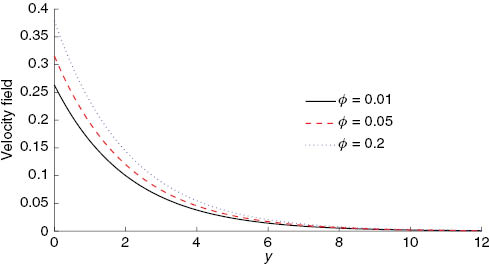
Influence of the nanofluid volume concentration φ on the velocity field (41) with ρ_s=8933, ρ_f=997.1, α=0.1, κ=0.7, and t=π fixed.

Figure 2:

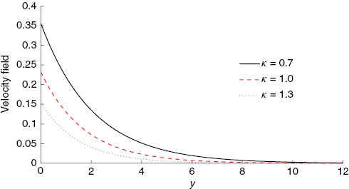
Influence of the porosity parameter κ on the velocity field (41) with ρ_s=8933, ρ_f=997.1, α=0.1, φ=0.1, and t=π fixed.

Figure 3:

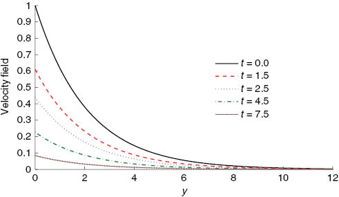
Influence of the time t on the velocity field (41) with ρ_s=8933, ρ_f=997.1, α=0.1, φ=0.1, κ=1, and t=π fixed.

Figure 4:

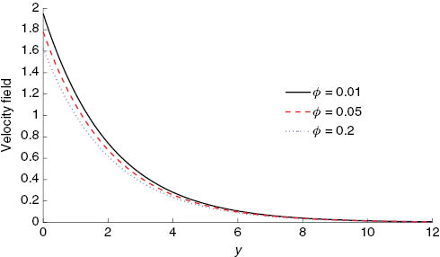
Influence of the nanofluid volume concentration φ on the velocity field (49) with ρ_s=8933, ρ_f=997.1, α=0.2, κ=0.7, and t=π fixed.

The influence of the nanofluid particles on the structure of the flow model is described in Figure 1. The graphs are plotted for copper–water nanofluid and it is clear from the figure that an increase in φ caused an increase in fluid velocity. These profiles are in agreement with physical-based nanofluids. Moreover, the velocity attains its maximum value near the surface but gradually decreases to zero at the free stream far away from the plate satisfying the boundary conditions, thus supporting the validity of the obtained results.

Figure 2 has been plotted to show the influence of the porosity of the porous medium κ on the velocity field (41). As anticipated, with an increase in the porosity of the porous medium causes an increase in the drag force and hence the velocity decreases.

The graphical behaviour of the travelling wave solution (41) for varying values of time t is shown in Figure 3. This figure depicts that the velocity decreases as the time increases. Clearly, the variation of velocity is observed for 0≤t≤7.5. For t>7.5, the velocity profile remains the same. In other words, we can say that the steady-state behaviour for the velocity is achieved for t>7.5.

In Figure 4, the group-invariant solution (49) is plotted for the varying values of the nanofluid volume concentration parameter φ. With the increase in φ the velocity profile decreases. This in turn decreases the thickness of the momentum boundary layer.

10 Conclusions

In this article, we have focused on highlighting the study of a non-Newtonian nanofluid flow model. The porous medium is also taken into consideration. The governing PDE of the non-Newtonian model along with nanoparticles is solved by employing the group theoretical and compatibility approach. The classically invariant solutions are formulated in the form of exponential functions. Furthermore, the conservation laws for the governing nonlinear PDE are also derived by employing the Ibragimov method. The importance of constructing the conservation laws has been discussed in the introduction.

The physical mechanism in the problem is diffusion. The fluid velocity is generated by the no-slip boundary condition when the plate is impulsively set in motion with a time-dependent velocity and diffuses in the direction towards the axis of the flow. This causes the velocity profiles to flatten out and the shear stress across the medium to steadily decrease and vanish as t→∞. The model has some features in common with the classical Stokes’ model for flow induced in a half-space of viscous fluid when a plate is impulsively set in motion. However, the present study can be described as a generalised Stokes’ flow for which the plate is impulsively set in motion with some time-dependent velocity which cannot be prescribed arbitrarily but depends on the physical parameters of the flow model. The results presented in this paper will now be available for experimental verification of the same type of nonlinear boundary value problems. It should be remarked that the flow model for this particular study has not been solved earlier by any traditional numerical approach.

References

[1] G. G. Stokes, Tran. Camb. Philos. Soc. 9, 1880 (1850).Suche in Google Scholar
[2] N. Tokuda, J. Fluid Mech. 33, 672 (1968).10.1017/S0022112068001606Suche in Google Scholar
[3] V. M. Soundalgekar, Rheol. Acta 13, 177 (1981).10.1007/BF01520872Suche in Google Scholar
[4] C. Fetecáu, D. Vieru, and C. Fetecáu, Int. J. Non-Linear Mech. 43, 457 (2008).10.1016/j.ijnonlinmec.2007.12.022Suche in Google Scholar
[5] R. Penton, J. Fluid Mech. 31, 819 (1968).10.1017/S0022112068000509Suche in Google Scholar
[6] K. R. Rajagopal, Int. J. Non-Linear Mech. 17, 369 (1982).10.1016/0020-7462(82)90006-3Suche in Google Scholar
[7] K. R. Rajagopal and T. Y. Na, Acta Mech. 48, 233 (1983).10.1007/BF01170422Suche in Google Scholar
[8] C. Fetecau and C. Fetecau, Int. J. Non-Linear Mech. 38, 1539 (2003).10.1016/S0020-7462(02)00117-8Suche in Google Scholar
[9] C. Fetecau, C. Fetecau, and M. Rana, Z. Naturforsch. 66a, 753 (2011).10.5560/zna.2011-0044Suche in Google Scholar
[10] S. Choi, ASME Int. Mech. Eng. Congress Expo. 66, 99 (1995).Suche in Google Scholar
[11] S. U. S. Choi, Z. G. Zhang, W. Yu, F. E. Lockwood, and E. A. Grulke, Appl. Phys. Lett. 79, 2252 (2001).10.1063/1.1408272Suche in Google Scholar
[12] H. Masuda, A. Ebata, K. Teramae, and N. Hishinuma, Netsu Bussei. 7, 227 (1993).10.2963/jjtp.7.227Suche in Google Scholar
[13] J. A. Eastman, S. U. S. Choi, S. Li, W. Yu, and L. J. Thompson, Appl. Phys. Lett. 78, 718 (2001).10.1063/1.1341218Suche in Google Scholar
[14] S. Lee, S. U. S. Choi, S. Li, and J. A. Eastman, Trans. ASME, J. Heat Transf. 122, 280 (1999).10.1115/1.2825978Suche in Google Scholar
[15] X. Wang, X. Xu, and S. U. S. Choi, J. Thermophys. Heat Transf. 13, 474 (1999).10.2514/2.6486Suche in Google Scholar
[16] P. Keblinski, S. R. Phillpot, S. U. S. Choi, and J. A. Eastman, Int. J. Heat Mass Transf. 45, 855 (2002).10.1016/S0017-9310(01)00175-2Suche in Google Scholar
[17] J. Buongiorno, ASME J. Heat Transf. 128, 240 (2006).10.1115/1.2150834Suche in Google Scholar
[18] S. Nadeem, R. Ul Haq, and Z. H. Khan, J. Taiwan Inst. Chem. Eng. 45, 121 (2014).10.1016/j.jtice.2013.04.006Suche in Google Scholar
[19] M. Ramzan and M. Bilal, PLoS One 10, (2015), doi:10.1371/journal.pone.0124929.Suche in Google Scholar PubMed PubMed Central
[20] A. K. Santra, S. Sen, and N. Chakraborty, Int. J. Thermal Sci. 48, 391 (2009).10.1016/j.ijthermalsci.2008.10.004Suche in Google Scholar
[21] N. Putra, W. Roetzel, and S. K. Das, Heat Mass Tran. 39, 775 (2003).10.1007/s00231-002-0382-zSuche in Google Scholar
[22] R. Ellahi, M. Raza, and K. Vafai, Math. Comput. Model. 55, 1876 (2012).10.1016/j.mcm.2011.11.043Suche in Google Scholar
[23] M. S. Kandelousi and R. Ellahi, Z. Naturforsch. 70, 115 (2015).10.1515/zna-2014-0258Suche in Google Scholar
[24] M. Sheikholeslami and R. Ellahi, Appl. Sci. 5, 294 (2015).10.3390/app5030294Suche in Google Scholar
[25] R. Ellahi, M. Hassan, and A. Zeeshan, Int. J. Heat Mass Transf. 81, 449 (2015).10.1016/j.ijheatmasstransfer.2014.10.041Suche in Google Scholar
[26] M. Sheikholeslami, D. D. Ganji, M. Y. Javed, and R. Ellahi, J. Magn Magn Mater. 374, 36 (2015).10.1016/j.jmmm.2014.08.021Suche in Google Scholar
[27] R. Ellahi, Appl. Math. Model. 37, 1451 (2013).10.1016/j.apm.2012.04.004Suche in Google Scholar
[28] R. Ellahi, M. Hassan, and A. Zeeshan, IEEE Trans. Nanotechnol. 14, 726 (2015).10.1109/TNANO.2015.2435899Suche in Google Scholar
[29] N. S. Akbar, M. Raza, and R. Ellahi, J. Magn Magn Mater. 381, 405 (2015).10.1016/j.jmmm.2014.12.087Suche in Google Scholar
[30] Y. Lin, L. Zheng, and X. Zhang, Int. J. Heat Mass Transf. 77, 708 (2014).10.1016/j.ijheatmasstransfer.2014.06.028Suche in Google Scholar
[31] Y. Lin, L. Zheng, X. Zhang, L. Ma, and G. Chen, Int. J. Heat Mass Transf. 84, 903 (2015).10.1016/j.ijheatmasstransfer.2015.01.099Suche in Google Scholar
[32] Y. Lin, L. Zheng, and G. Chen, Powder Tech. 274, 324 (2015).10.1016/j.powtec.2015.01.039Suche in Google Scholar
[33] G. W. Bluman and S. Kumei, Symmetries and Differential Equations, Springer, New York 1989.10.1007/978-1-4757-4307-4Suche in Google Scholar
[34] P. J. Olver, Application of Lie Groups to Differential Equations, Graduate Texts in Mathematics, Vol. 107, Springer-Verlag, New York 1993.10.1007/978-1-4612-4350-2Suche in Google Scholar
[35] R. L. Fosdick and K. R. Rajagopal, Proc. R. Soc. Lond. Ser. A 339, 351 (1980).Suche in Google Scholar
[36] M. Pakdemirli and B. S. Yilbas, Int. J. Non-Linear Mech. 41, 432 (2006).10.1016/j.ijnonlinmec.2005.09.002Suche in Google Scholar
[37] T. Aziz, F. M. Mahomed, and A. Aziz, Int. J. Non-Linear Mech. 47, 792 (2012).10.1016/j.ijnonlinmec.2012.04.002Suche in Google Scholar
[38] G. Saccomandi, Int. J. Eng. Sci. 29, 645 (1991).10.1016/0020-7225(91)90069-FSuche in Google Scholar
[39] K. Das, Appl. Math. Comput. 221, 547 (2013).10.1016/j.amc.2013.06.073Suche in Google Scholar
[40] T. Aziz, A. Fatima, A. Aziz, and F. M. Mahomed, Z. Naturforsch. 70, 483 (2015).10.1515/zna-2015-0099Suche in Google Scholar
[41] M. Pakdemirli, Y. Aksoy, M. Yürüsoy, and C. M. Khalique, Acta Mech. Sin. 24, 661 (2008).10.1007/s10409-008-0172-zSuche in Google Scholar
[42] C. Wafo Soh, Commun. Nonlinear Sci. Numer. Simul. 10, 537 (2005).10.1016/j.cnsns.2003.12.008Suche in Google Scholar
[43] A. G. Fareo and D. P. Mason, Commun. Nonlinear Sci. Numer. Simul. 18, 3298 (2013).10.1016/j.cnsns.2013.04.019Suche in Google Scholar
[44] C. M. Khalique, J. Appl. Math. 2013, 741780 (2013).Suche in Google Scholar
[45] A. Sjoberg, Appl. Math. Comput. 184, 608 (2007).10.1016/j.amc.2006.06.059Suche in Google Scholar
[46] R. Naz, F. M. Mahomed, and D. P. Mason, Appl. Math. Comput. 205, 212 (2008).10.1016/j.amc.2008.06.042Suche in Google Scholar
[47] D. M. Mothibi and C. M. Khalique, Symmetry 7, 949 (2015).10.3390/sym7020949Suche in Google Scholar
[48] T. Aziz, F. M. Mahomed, and D. P. Mason, Int. J. Non-Linear Mech. 78, 142 (2016).10.1016/j.ijnonlinmec.2015.01.003Suche in Google Scholar
[49] A. Fatima and F. M. Mahomed, Int. J. Non-Linear Mech. 67, 95 (2014).10.1016/j.ijnonlinmec.2014.08.013Suche in Google Scholar
[50] N. H. Ibragimov, J. Math. Anal. Appl. 333, 311 (2007).10.1016/j.jmaa.2006.10.078Suche in Google Scholar
©2016 by De Gruyter
Artikel in diesem Heft
- Frontmatter
- Decay Mode Solutions for the Supersymmetric Cylindrical KdV Equation
- Cooling of Moving Wavy Surface through MHD Nanofluid
- Parallel Plate Flow of a Third-Grade Fluid and a Newtonian Fluid With Variable Viscosity
- Flow of a Micropolar Fluid Through a Channel with Small Boundary Perturbation