Optimal Macroeconomic Policy in Nonlinear Models: A VSTAR Perspective
-
Vito Polito


Abstract
The paper describes a method to transform vector smooth transition autoregressions in a form that is particularly suitable for policy analysis, because it is of low-dimension and retains certainty-equivalence. Optimal rules are calculated with the state dependent coefficients approach, which allows linear methods to solve nonlinear problems. The methodology is applied to revisit interest rate and quantitative easing (QE) monetary policy in the United States during 1979–2018. The actual size of QE and duration of the zero lower bound are found close to those prescribed by the optimal policy, but not the timing and composition of QE. The methodology compares favourably against alternative optimization approaches based on linearization or numerical search.
1 Introduction
This paper describes a methodology for the analysis of optimal macroeconomic policy when the interaction between the economy and the policy sector is described by a widely-used class of nonlinear models: vector smooth transition autoregressions (VSTARs). VSTAR models have become increasingly popular in macroeconometrics given their ability to better describe data compared to linear models. In applied works VSTARs are often used for forecasting and to account for history dependence in the response of macroeconomic variables to shocks. While the econometric literature has long established methods for specification, estimation and structural analysis with VSTAR, no attention has been devoted so far to the analysis of policy. The present paper attempts to fill this methodological gap.
The proposed methodology is applied to evaluate the actual conduct and effects of conventional (interest rate) monetary policy and large scale asset purchase programs, frequently referred to as quantitative easing (QE), undertaken by the Fed since 2008 against the framework obtained from the optimal policy. This seems a pertinent application of the VSTAR, given the extent of nonlinearity displayed by macroeconomic data of the United States over the last 40 years and, particularly, by the federal funds rate and the Fed’s balance sheet in the decade after the onset of the Great Recession. According to this analysis, the size of QE undertaken by the Fed and the duration of the zero lower bound (ZLB) are not too dissimilar from those prescribed by the optimal policy, but there are differences in terms of the timing and composition of QE.
Given a welfare function and a structural model of the economy, monetary policy could be evaluated considering commitment to a rule derived by maximising welfare subject to the model. Quantitative policy evaluation based on structural models is however not problem free. Above all it is often difficult to get agreement on how to specify a structural model of the economy. This is true even for well-established structural models such as the Smets and Wouters (2003) model, as argued by Chari et al. (2009). Challenges compound when dealing with QE because structural models tend to abstract from large changes in the economy, assuming parameters and sources of shocks to be constant over time and known by policy makers. These issues are particularly noteworthy for quantitative analyses dealing with the significant instabilities and jumps in the data of the last 25 years, as well as the asymmetric nature of the ZLB. An alternative solution is to quantify policy based on a nonlinear vector autoregression model of the economy. Its main attraction is that, whatever the structural model, a close approximation is given by a vector autoregression representation. Although the resulting policy would not be first best compared with using a correct structural model, it would be a simple and transparent way to proceed. It would also provide a useful benchmark against which to compare any other policy decisions, and it has the advantage of being easily automated.
Against this backdrop, the paper makes two methodological contributions. To better highlight these, it is useful to recap how the effects of systematic changes in policy are evaluated when using a linear VAR. In a VAR all (policy and non-policy) variables are endogenous. To quantify the impact of a systematic change in policy, the VAR needs to be transformed into a VARX in which the policy variables are exogenous. This is achieved through a block decomposition separating the vector of policy instruments from the remaining variables in the VAR. Depending on whether the policy variables are ordered first or last, at least two possible VARX representations can be derived, see for example Sack (2000) and Stock and Watson (2001). These VARX representations differ in terms of the timing assumption about the economy response to a policy change, which can be either with a lag (A1) or contemporaneous (A2). If the objective function of the decision maker is quadratic, optimal policy can then be calculated as a linear quadratic regulator (LQR) problem using either of these two VARX models. Crucially, both A1 and A2 satisfy certainty equivalence, solving the LQR problem regardless of the particular sequence of disturbances. For this reason solutions can be computed using linear dynamic programming based on Riccati equation iteration, as shown in Ljungqvist and Sargent (2018).
The first methodological contribution refers to the derivation of a VSTARX model suitable for optimal policy analysis from a reduced-form VSTAR. It is shown that when using either A1 or A2 in a VSTAR, differences between the two VSTARX representations go well beyond the timing of interaction among variables. A1 gives rise to a nonlinear quadratic regulator (NLQR) problem that is high dimensional and no longer consistent with certainty equivalence. In contrast, A2 has the advantage of delivering a small dimensional NLQR problem compatible with certainty equivalence.
The second methodological contribution refers to the calculation of optimal decision rules that solve the NLQR problem. This consists of employing state dependent coefficient (SDC) factorization to transform the nonlinear VSTARX into an affine model with SDC matrices. As a result, the NLQR problem becomes isomorphic to the LQR. Under A2, the problem is also low dimensional and certainty equivalent, and it can be solved with linear dynamic programming methods. The solution yields an optimal feedback rule with time-varying coefficients that can be combined with the VSTARX to construct the reduced-from VSTAR under the optimal rule.
Of course, any nonlinear model could be linearized and then analyzed with LQR. However, as well as providing solutions that are not globally valid, linearization assumes away crucial features of macroeconomic data, such as asymmetries, threshold effects and large transitional changes. A VSTAR could well capture these features, but the LQR solution would disregard them, potentially resulting in incorrect and/or inefficient decision making. Alternatively, policy analysis could be carried out with numerical methods. While these can deliver globally valid solutions without disregarding nonlinearity, their main drawback is that they are computationally intensive and their effectiveness in finding the optimal solution is often impeded when nonlinearity is significant. The proposed SDC method has the advantage of accounting for nonlinearity while being computationally simple and easy to understand given his similarity to the LQR. It also allows the use of dynamic programming, one of the most powerful tools for solving decision problems in economics.
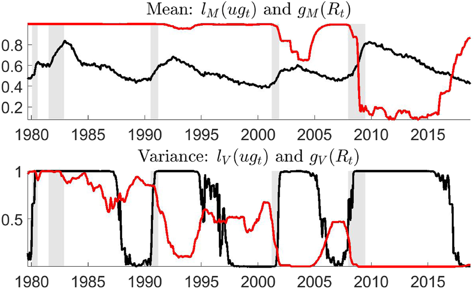
The proposed methodology is applied using a VSTAR estimated with maximum likelihood on monthly data for the United States during 1979:8-2018:10 (Figure 1). In the benchmark specification, the model includes seven variables: credit spread, inflation, industrial production, unemployment rate, the federal funds rate, and total assets held by the Fed split between Treasury and privately-held securities.[1] The policy analysis therefore accounts for the macroeconomic effects of changes in both the size and composition of the Fed’s balance sheet as well as the ZLB. Nonlinearity in the mean and variance of the VSTAR is captured by allowing the coefficients to change during periods of economic slack and when the federal funds rate is near to the ZLB. It is shown that the estimated VSTAR can well capture nonlinearities in the data (Figure 2) and provides a plausible description of the response of the three policy instruments to shocks at different times of the United States’s monetary history (Figure 3).
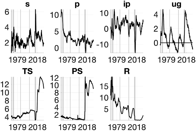
Macroeconomic data, United States 1979:8-2018:10. NBER recessions in grey. All variables are in percentage.
Transition probabilities l i (ug t ) (black) and g i (R t ) (red), in the mean i = M and covariance matrix i = V of the estimated VSTAR. NBER recessions in grey.
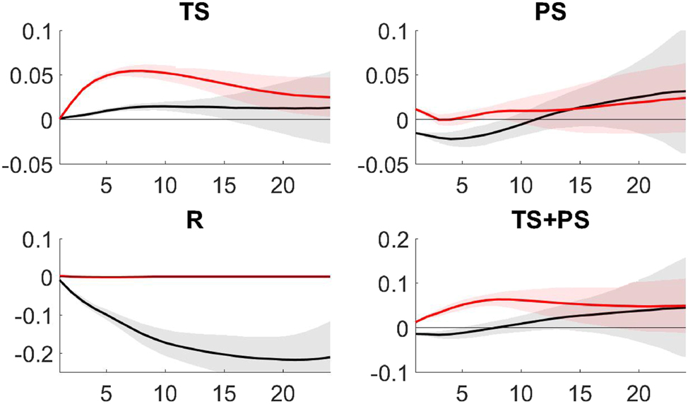
Median and two standard deviation confidence bands of IRFs of policy instruments to a credit shock during normal times (black) and the ZLB period (red). All variables are in percentage.
The estimated VSTAR is used to evaluate how far from optimal were the actual interest rate policy and QE undertaken by the Fed in the decade after the onset of the Great Recession. By focusing exclusively on the post-2008 period, the policy analysis avoids the substantial macroeconomic shifts that occurred between the pre- and post-Great Recession periods. The optimal VSTAR is obtained from the joint optimization of all monetary policy instruments under alternative specifications of the Fed’s preferences. The evaluation considers three different dimensions: the gains from optimization; the response of monetary policy to shocks; and counterfactual simulations. According to these results, the actual QE and ZLB policy were not too far from those otherwise prescribed by the optimal analysis. In particular, the joint optimization of the monetary policy instruments since 2008 would have resulted in: (i) Reduction of the average unemployment rate by 0. 33 %. This is about one-third of that measured for the actual QE policy relative to a scenario of no-QE (0.97 % ) (Table 1); (ii) Responses of QE to credit shocks very similar to those obtained under the actual policy, particularly beyond the very short-run horizon (three months) (Figures 4 and 5); (iii) Increase in size of the Fed’s balance sheet as a proportion to GDP (between 17.98 and 19.33 % ) in line with that observed from the data (17.96). There are however differences in the timing and composition of QE, as according to the optimal policy larger purchases of Treasury securities should have occurred during the first phase of QE (Figure 6 and Table 3); (iv) Average ZLB duration (between 68 and 73 months) close to that observed from the data (96 months), in contrast with the view that the ZLB should have terminated much earlier (after 26 months) supported by the standard Taylor rule, see Williamson (2015) (Table 2).
Gains from monetary policy optimization computed from the VSTAR.
| Items in the loss function | Loss | Stabilization | ||||||
|---|---|---|---|---|---|---|---|---|
|
|
|
|
|
|
V | G |
|
|
| Policy | Baseline: υ p = υ ug = υΔTS = υΔPS = υΔR = 1 | |||||||
| Actual | 1.24 | 5.46 | 0.02 | 0.05 | 0.38 | 7.15 | ||
| Optimal | 1.05 | 5.33 | 0.05 | 0.25 | 0.39 | 7.08 | 0.98 | 0.26a |
| No-QE | 2.47 | 5.55 | 0.02 | 0.00 | 0.00 | 8.05 | 11.15 | 0.95b |
| Weights II: υ p = 0.5, υ ug = υΔTS = υΔPS = υΔR = 1 | ||||||||
| Actual | 1.24 | 5.46 | 0.02 | 0.05 | 0.38 | 6.53 | ||
| Optimal | 1.14 | 5.29 | 0.06 | 0.19 | 0.37 | 6.47 | 0.84 | 0.23a |
| NoQE | 2.47 | 5.55 | 0.02 | 0.00 | 0.00 | 6.81 | 4.11 | 0.53b |
| Weights III: υ ug = 0.5, υ p = υΔTS = υΔPS = υΔR = 1 | ||||||||
| Actual | 1.24 | 5.46 | 0.02 | 0.05 | 0.38 | 4.42 | ||
| Optimal | 1.03 | 5.40 | 0.05 | 0.22 | 0.38 | 4.39 | 0.67 | 0.24a |
| No-QE | 2.47 | 5.55 | 0.02 | 0.00 | 0.00 | 5.27 | 16.18 | 1.31b |
| Weights IV: υ ug = υ p = 1, υΔTS = υΔPS = υΔR = 0.5 | ||||||||
| Actual | 1.24 | 5.46 | 0.02 | 0.05 | 0.38 | 6.92 | ||
| Optimal | 0.97 | 5.28 | 0.06 | 0.38 | 0.46 | 6.70 | 3.16 | 0.47a |
| No-QE | 2.47 | 5.55 | 0.02 | 0.00 | 0.00 | 8.03 | 13.82 | 1.05b |
| Weights V: υ ug = υ p = υΔR = 1, υΔTS = υΔPS = 0.5 | ||||||||
| Actual | 1.24 | 5.46 | 0.02 | 0.05 | 0.38 | 6.92 | ||
| Optimal | 0.97 | 5.28 | 0.06 | 0.38 | 0.46 | 6.70 | 3.16 | 0.47a |
| No-QE | 2.47 | 5.55 | 0.02 | 0.00 | 0.00 | 8.03 | 13.82 | 1.05b |
| Weights VI: υ ug = υ p = υΔTS = υΔPS = 1, υΔR = 0.5 | ||||||||
| Actual | 1.24 | 5.46 | 0.02 | 0.05 | 0.38 | 7.14 | ||
| Optimal | 1.04 | 5.32 | 0.07 | 0.25 | 0.39 | 7.03 | 1.44 | 0.32a |
| No-QE | 2.47 | 5.55 | 0.02 | 0.00 | 0.00 | 8.03 | 11.16 | 0.95b |
| Average (across weights) | ||||||||
| Actual | 1.24 | 5.46 | 0.02 | 0.05 | 0.38 | 6.51 | ||
| Optimal | 1.03 | 5.32 | 0.06 | 0.28 | 0.41 | 6.40 | 1.71 | 0.33a |
| No-QE | 2.47 | 5.55 | 0.02 | 0.00 | 0.00 | 7.37 | 11.71 | 0.97b |
-
G is the stabilization gain;
Median and two standard deviation confidence bands of IRFs to a credit shock during the ZLB period under the actual (red) and the optimal (blue) policy. All variables are in percentage.
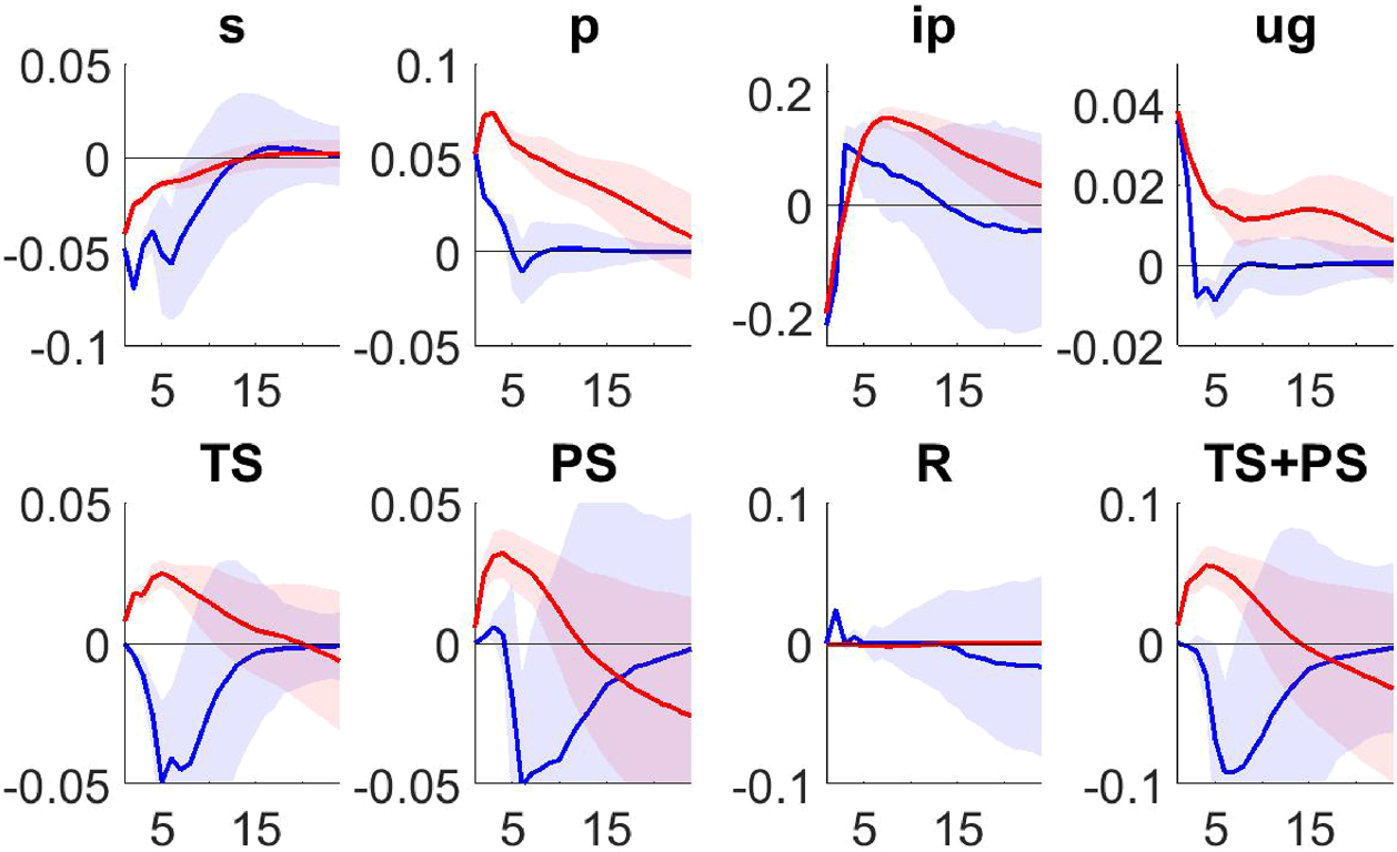
Median and two standard deviation confidence bands of IRFs to a supply-type shock during the ZLB period under the actual (red) and the optimal (blue) policy. All variables are in percentage.
Counterfactual simulations of interest rate and QE policy in the United States. ‘A’ denotes the actual paths; ‘O2’, ‘O3’ and ‘O4’ the counterfactual paths under the inflation targets of 2, 3 and 4 %, respectively. All variables are in percentage.
Duration of the ZLB period under the actual and optimal policy.
| Number of months when | ||||
|---|---|---|---|---|
| R less than: | ||||
| 0.25 | 0.5 | 0.75 | 100 | |
| Actual policy | ||||
| 85 | 97 | 100 | 104 | |
| Optimal policy | ||||
|
|
26 | 55 | 87 | 104 |
|
|
51 | 72 | 74 | 84 |
|
|
71 | 73 | 73 | 75 |
-
Source: Author’s calculations. See main text for more details.
To gauge some indication on the quality of the quantitative performance of the proposed methodology, the results are compared with those from three alternative optimization approaches. The first is based on linearization. The other two, model predictive control and direct search, are nonlinear optimizers that rely upon numerical search using the VSTARX from A1. The proposed methodology is found to deliver faster and larger optimization gains compared to any of these alternatives (Table 5).
Two possible caveats on the quantitative results should be noted. The first concerns the specification of the Fed preferences. Economic theory offers little guidance on this since structural models with QE include heterogeneous households, a feature which prevents the identification of a unique micro-founded objective function for the central bank. Optimal policy is computed in this paper assuming a standard quadratic loss function in inflation and unemployment, as in Sims et al. (2023) and consistently with the Fed’s dual mandate of price stability and full employment. For robustness, alternative specifications are appraised by varying the loss function parameters. The second caveat is that, in principle, counterfactual analysis with a VSTAR enters the territory of the Lucas (1976) critique. While its quantitative significance is often debated, see Rudebusch (2005) and Sims and Zha (2006), to guard against it the loss function is expanded including penalties for changes in the policy instruments. This ensures that the counterfactual policy simulations are close to the actual data, making them less susceptible to the critique. It is also shown that the simulated paths under the optimal policy are within the range of macroeconomic forecasts from professional survey data (Table 4). In addition, the analysis mainly focuses on the post-2008 period, thus avoiding the change in policy regime relative to the pre-2008 period.[2]
1.1 Related Literature
The paper makes several contributions to the literature. The methodological part is related to the research on nonlinear time series modelling, which has long established methods for the specification, estimation and structural analysis of VSTAR, see Granger et al. (1993), Dijk et al. (2002) and Martin et al. (2013). The paper complements this literature, tackling a different task, the analysis of systematic policy. The methodological part also contributes to the macroeconomic literature on optimal decision analysis. As mentioned above, the predominant paradigm here is still the LQR, which applies to linear economic environments, see Ljungqvist and Sargent (2018). The approach adopted in the paper illustrates how to bring the same LQR techniques to nonlinear economic models.
The paper also contributes to three strands of applied econometrics. The first is the analysis of the wider effects of QE and the ZLB based on VAR or semi-structural models. Examples include Lenza et al. (2010), Kapetanios et al. (2012), Gambacorta et al. (2014), Dahlhaus et al. (2018). These works evaluate what the unconventional monetary policy undertaken by the Fed since the Great Recession managed to achieve relative to a scenario of no-intervention. The paper complements this literature evaluating what the actual QE and ZLB policy could have achieved, using as reference the framework from the optimal policy. The second is the applied literature on macroeconomic asymmetries and the transmission channels of QE and the ZLB, typified by the works of Guerrieri and Iacoviello (2017) and Sims and Wu (2020); Sims et al. (2023). The present paper shares with these works a similar emphasis on the dual source of nonlinearity, from the economy and the policy sectors, but for the purpose of empirical analysis. The third is the literature using VSTAR-type models to account for nonlinearity in macroeconomic time series, whose applications spans from business cycle, Terasvirta and Anderson (1992), international spillovers, Gefang and Strachan (2009), fiscal policy, Auerbach and Gorodnichenko (2012) (conventional) monetary policy, Dahlhaus (2017), and credit markets, Atanasova (2003). The paper contributes to this literature using a VSTAR for the analysis of QE and the ZLB.
There is a growing literature that develops dynamic stochastic general equilibrium (DSGE) models to study monetary policy when the short term interest rate is constrained by the zero lower bound and the Fed embarks on QE. This literature considers actual and/or optimal QE intervention targeting either private assets, through outright purchases or collateralized short-term loans, as for example in Del Negro et al. (2017), or long term government bonds, as for example in Sims and Wu (2021). The present paper contributes to this literature considering in a reduced form framework the design of QE programmes that simultaneously involve private securities and government bonds purchases. Being reduced form, the analysis is unable to explain the economic mechanisms that may explain why each type of QE is required and desired. It is also silent about the distortions that these purchases may induce on private sector decisions. The main advantage of taking a reduced form approach is that it facilitates the empirical analysis of the effects of conventional and unconventional monetary policy despite the large data instabilities occurred during both the build-up of QE and its first phase of unwinding since 2015, allowing to compare and contrast the effects of different types of asset purchases, how these policies interact with each other and quantify their outcomes in terms of stabilization gains.
This paper is also related to a recent literature that uses DSGE models to conduct counterfactual policy analysis in reduced-form or semi-structural frameworks that aim to be robust to the Lucas critique, see, Barnichon and Mesters (2023), Beraja (2023) and McKay and Wolf (2023). While the methodology in this paper does not explicitly aim to insulate policy analysis from the Lucas critique, it is implemented in a way that attempts to minimize the quantitative relevance of the critique. The methodologies in this recent literature have also limited applicability. Beraja (2023)’s approach only applies to DSGE models that can be linearized, thereby excluding nonlinearities induced by ZLB or leverage constraints that typically features DSGE models with QE. Barnichon and Mesters (2023)’s sufficient statistics cannot be used to compute the optimal policy if there is not enough empirical evidence to estimate the responses to all policy news shocks (The authors also discuss circumstances in which their optimal policy perturbation approach is not applicable to nonlinear models). The identification result of McKay and Wolf (2023) also relies on linearity and is not suited to study change in the steady state. In contrast, the approach proposed in this paper has the advantage of being applicable to a much broader set of nonlinearities and policy experiments, as demonstrated in the empirical application.
The paper is organized as follows. Section 2 describes the reduced-form VSTAR and the two VSTARX representations under A1 and A2. Section 3 illustrates the SDC method and derives the VSTAR under control. Sections 4 and 5 present the results from the estimated VSTAR and the analysis of optimal policy, respectively. Section 6 concludes with a summary. Supplementary material and robustness results are in Appendix.
2 The VSTAR Model
2.1 Reduced Form
Let
where y0 is given; λ
j
are vectors of constant coefficients of dimensions n × 1;
where Ω
j
are symmetric matrices of coefficients, j = 1, …, 4. The terms
The VSTAR model in (1)-(2) provides a natural framework to study monetary policy in non-linear macroeconomic environments. The idea of considering dual nonlinearity, from the economy and the policy sectors, is not new. It features in recent works of Guerrieri and Iacoviello (2017) and Sims and Wu (2020); Sims et al. (2023) based on DSGE models where nonlinearity stems from the private sector, due to collateral constraints on borrowing, and from the policy sector, due to the ZLB. The specified VSTAR shares with these works a similar emphasis on the dual nonlinearity, with the purpose however of evaluating its significance for empirical analysis.
2.2 VSTARX Form
The VSTAR in (1)-(2) is a reduced form, suitable for econometric estimation and dynamic analysis like forecasting. The coefficients in the equations for the policy instruments describe the so-called actual policy rules. The coefficient in the equations for the economy vector describe how the economy evolves over time subject to the actual policy rule.
To quantify the impact of a change in policy, the coefficients in the equations for the instruments need to be replaced with those from another policy rule, either ad-hoc or optimal in some sense. This requires transforming the VSTAR into a VSTARX where the policy variables are treated as exogenous. As in a VAR, this transformation requires only a zero block factorization (sufficient condition) of the reduced-form covariance matrix, to separate the policy vector from the economy vector. Thus, there are (at least) two possible representations depending on whether the policy variables are ordered first or last.[3]
To elucidate the structure of, and the differences between, these two VSTARX forms, consider partitioning the mean equation (1) to separate the economy from the policy instruments.[4] The covariance matrix (2) can be conformably partitioned as:
Under A1, the economy reacts with a lag to a change in policy, requiring Ω xut = 0 in (3).
Under A2, the economy reacts within the same period, thus requiring Ω uxt = 0.
To start, consider applying A1 and A2 to the VAR obtained after all transition functions in the VSTAR are set equal to zero. This yields:
The above are two VARX models in which the vector of policy instruments u enters on the right side as an exogenous variable.[5] These two VARX differ in terms of the interaction between the economy and the policy instruments, being with a lag under A1 and contemporaneous under A2. Using either of them as constraint for optimization makes no difference in terms dimensionality, since a change in the policy vector has a direct effect on the endogenous variables only through the time-invariant coefficients
Applying A1 to the VSTAR, yields:
where
Conversely, applying A2 to the VSTAR yields:
where
The nonlinear dynamic of y t under both (4) and (6) describes a VSTAR with exogenous variables, i.e. a VSTARX, since the policy vector u t enters on the right side of both models as an exogenous variable.[6] Therefore, both (4) and (6) can be used to represent the nonlinear economy constraint faced by a regulator in charge of setting u t . When the objective of the regulator is approximated by a quadratic function, the resulting problem is referred to as the NLQR problem.
It is useful to point out the differences between (4)-(5) and (6)-(7) due A1 and A2. The VSTARX in (4)-(5) corresponds to the equations for the economy vector x t in the reduced-form VSTAR (1)-(2). In contrast, the VSTARX in (6)-(7) is obtained by extrapolating from the reduced-form covariance matrix (3) the contemporaneous response of the economy to policy and then incorporating this into the systematic part of x t .
There are three further differences, specific to the nonlinear nature of the VSTAR. The first refers to the response coefficient of the economy variables x
t
to changes in the policy vector u
t
. In (4) this reflects the nonlinearity in the mean of the VSTAR as it is given by
Both (4)-(5) and (6)-(7) can be employed as constraints in a NLQR problem. The VSTARX in (4)-(5) has however two main drawbacks. First, the NLQR solution becomes highly dimensional. This is because the coefficients in (4) depend on the lagged value of the policy vector, the variable set by the regulator. Thus changes in u
t
affect on impact the entire system through Γ
j
and
The empirical evidence on optimal monetary policy analysis based VAR, finds that the two timing protocols of A1 and A2 in general do not result in large quantitative differences, see Polito and Wickens (2012). Given the methodological advantages highlighted above, the NLQR problem is thus specified and solved in the next section using the VSTARX based on A2 in (6)-(7). A further reason for preferring A2 is that a reduced-form policy experiment could miss the timing of the policy impact on the economy, as forward-looking agents in the private sector can be expected to incorporate information about the implementation of policy at the time of announcement, see Dahlhaus et al. (2018). As also argued by Stock and Watson (2001), A2 minimizes this shortcoming by at least allowing the economy to react within the same period of a change in policy.[7]
3 Optimal Policy
3.1 Specification
The problem of setting optimal policy is specified as a closed-loop regulator determining the sequence of policy instruments
where E0 denotes mathematical expectation conditional on information at t = 0;
The above NLQR problem has not closed-form solution. One option is to linearize (6) so that the NLQR problem effectively becomes a LQR and a closed-form solution can be calculated with linear dynamic programming, for example using Riccati equation iteration as in Ljungqvist and Sargent (2018). The alternative is to solve the problem numerically using the nonlinear model of the economy as it is or a higher-order approximation. Linearization would somehow be inconsistent with the aim of this paper, i.e. studying the significance of macroeconomic nonlinearity for optimal policy analysis. The main drawback of numerical methods is that they can be computationally intensive and there is not guarantee about their optimization performance in highly nonlinear models. This is because direct search methods can easily default on local minima while gradient methods can quickly loose efficiency once differentiation becomes either intractable or very high dimensional due to nonlinearity. Luukkonen et al. (1988) show how to employ Taylor-series expansion of the transition function of the VSTAR to derive a polynomial approximation that can be used to test for nonlinearity in the data. With this approach, however, the economy constraint of the NLQR would remain still highly nonlinear, even when using a first-order approximation of the transition function.
The SDC method extends Riccati equation iteration used in LQR to the nonlinear case. This is done by approximating the NLQR problem into a sequence of one-period LQR problems that can be solved independently. The SDC method has the advantage of being numerically simpler than many other nonlinear optimization techniques, as well as being closely related to the well-understood Riccati equation method used for LQR. The SDC method is widely applied in engineering and data science.[9] The next subsections describe how to adapt it for optimal macroeconomic policy analysis with a VSTAR.
3.2 The SDC Method
Applying the SDC method to solve the NLQR problem of minimizing (8) subject to (6)-(7) requires two steps. The first consists of employing SDC factorization to transform the nonlinear model (6) into an affine structure with SDC matrices. As a result, the NLQR problem can be written in a form that is isomorphic to the LQR problem and it can be solved with linear dynamic programming techniques. The second step consists of solving the NLQR problem iterating on the resulting SDC solutions. This yields a feedback rule for the policy instruments with time-varying response coefficients that can be combined with the original constraint to derive the VSTAR under control.
3.2.1 Factorization
SDC factorization is typically used, outside economics, for solving (i) continuous time, (ii) deterministic NLQR problems, (iii) using the method of variation. The approach is adapted here for solving (i) discrete time, (ii) stochastic NLQR problems, (iii) using dynamic programming. To illustrate the logic of SDC factorization, consider the differential equation for an autonomous system, with fully observable state, nonlinear in the state and affine in the control:
Proceeding in a similar fashion, the nonlinear system in equation (6) can be factorized in terms of SDC matrices and rewritten as
for t ≥ 0, using:
with the upper part of Γ
t
, i.e. G12t, being given by (7).[11] Three results about the above SDC factorisation are worth highlighting. First, by construction the SDC factorization gives a representation of the model of the economy mathematically equivalent to VSTARX model in (6). Second, the SDC vectors
3.2.2 Solution
Following the SDC factorization, the closed-loop regulator problem consists of finding the sequence
This formulation of the NLQR problem is isomorphic to the LQR except for the objects
which is a linear feedback rule with time-varying coefficients, k t and K t .[13] This can be combined with the equations for the economy in SDC form in (9) as:
to recover a reduced-form model with time-varying coefficients:
where
and
4 Estimated VSTAR
4.1 Data
The VSTAR is estimated using aggregate monthly data for the United States from 1979:8 to 2018:10.[14] In the benchmark specification, the endogenous vector comprises seven variables: an indicator of credit risk, the spread between the Baa corporate rate and the 10-year treasury rate (s); the inflation rate (p), measured as the annual change in the personal consumption expenditures deflator; the annual growth rate of industrial production (ip); the difference between the actual and the natural rate of unemployment, the unemployment gap (ug); Treasury securities held by the Fed as a proportion to GDP (TS); private securities held by the Fed as a proportion to GDP (PS); and the federal fund rate (R).[15] The selected measure of credit risk is used as a proxy for financial conditions in the macroeconomy.[16] Inflation and the unemployment gap are used as indicators of the Fed targets of price stability and maximum employment, respectively, as in Williamson (2015). Industrial production is used as a proxy for aggregate output, following Sack (2000). The sum of TS and PS equals total assets held in the Fed’s balance sheet. Thus the VSTAR includes conventional and QE monetary policy tools, and can account for variation in both the size of the Fed’s balance sheet and the composition of its assets portfolio.
As in Gambacorta et al. (2014), the total size of the Fed’s balance sheet is used to proxy QE. The distinction between TS and PS captures the effects of QE on aggregate demand through the portfolio-balance and the credit channels, respectively, highlighted by the economic theory. Kuttner (2018) supports this distinction on the ground that it characterizes the conduct of QE in the United States since 2008, which involved large purchases of PS in the immediate aftermath of the Great Recession, and of TS afterwards.[17]
Figure 1 plots the data, with NBER recession periods highlighted in grey for reference. with NBER recessions highlighted in grey. Several clear irregularities are visible over the sample period, such as the large spikes in the credit risk, inflation, industrial production and unemployment gap; the asymmetric dynamics of the unemployment gap above and below zero; the large transitional changes in the two QE variables around the Great Recession; and the flat path of the federal fund rate while at the ZLB. It is the presence of these irregularities that motivates the use of a VSTAR.[18]
4.2 Specification
Variables are ordered as
Transition across states due to nonlinearity in the economy is modelled using a logistic function
To ensure positive definiteness on the variance covariance matrix in (2) and on its determinant, each matrix of coefficients Ω j is decomposed as
where D j is a lower triangular matrix, j = 1, …, 4.
4.3 Estimation
Given a sample of t = 1, …, T observations and the i.i.d. assumption on the disturbances v t , the log-likelihood function of the VSTAR in (1)-(2) conditional on the first q observations is formed as:
where Π is a vector collecting all VSTAR parameters in equations (1), (2) and (13). It is convenient to partition the vector of parameters as Π = [Π1, Π2], where Π1 = {λ1, Λ1(L), λ2, Λ2(L), λ3, Λ3(L), λ4, Λ4(L)} includes the linear coefficients in the conditional mean (1), while Π2 = {D1, D2, D3, D4, γ lM , γ lV , γ gM , γ gV } includes the coefficients pertinent to the covariance matrix and to the transition functions.
To establish the optimal lag length and estimate the model parameters, an algorithm similar to that used by Auerbach and Gorodnichenko (2012) is adapted to the VSTAR in equations (1), (2) and (13).[20] The algorithm exploits the possibility of writing the model in a linear form conditional on a subset of the parameters, thereby estimating the remaining parameters analytically. Thus, estimation involves repeating until convergence two sequential steps. The first consists of determining a draw of Π2. Conditional on Π2, the VSTAR is linear in the remaining parameters over the four states. In the second step the remaining parameters in Π1 can be determined analytically via generalized least squares and the log-likelihood can be evaluated from (14). The estimation is undertaken including up to 12 lags and the model fit evaluated using information criteria such as, Akaike (AIC), Hannan (HIC) and Schwarz (SIC), in both standard and normalised form. The model with one lag is the preferred specification according to almost any of the information criteria considered.[21] In Appendix E in Supplementary Material it is also shown that the proposed VSTAR specification yields a better fit of the data compared to several other VSTAR specifications often used in the applied macroeconomic literature.
Figure 2 plots the transition probabilities estimated from the VSTAR for the mean (top panel) and the covariance matrix (bottom panel) parameters. The black lines show the probability of the economy being,
4.4 Impulse Response Functions
IRF analysis with VSTAR is typically based on the algorithm of Koop et al. (1996), with shocks identified through Cholesky factorization of the covariance matrix Ω t . In a small-scale VAR the Cholesky decomposition yields structural shocks that can be easily reconciled with an economic interpretation. This is not necessarily the case in larger (and nonlinear) models like the estimated VSTAR. For this reason, IRF analysis is carried out in this paper by adapting the algorithm of Koop et al. (1996) to include sign restrictions.[24] To formulate a benchmark, the restrictions are set to identify a credit-type shock that on impact yields macroeconomic dynamics similar to those observed in the United States after 2008, leaving entirely unrestricted the policy variables. This shock is such that both the spread and the unemployment gap increase while inflation and industrial production decrease at the one month horizon.[25] To evaluate the different responses of the policy instruments during periods when either conventional monetary policy or QE is active, the IRFs are computed using as starting values for y t the averages over two sub-samples of equal size. The first is from 1994:6 to 2001:5. This is referred to as the normal times, covering a period when the federal funds rate is well above the ZLB. The second includes observations for the ZLB period, from 2009:1 to 2015:12.
Figure 3 displays the responses of the three policy instruments plus the total size of the Fed’s balance sheet (TS + PS) to the identified credit shock over 24 months. In each panel, the black lines denote the responses during normal times, the red lines the responses in the ZLB period and the shaded areas denote two standard deviations confidence bands. The response of the policy instruments mimics that of expansionary monetary policy intervention at different periods of the United States’ economic history. In normal times the shock leads to a reduction of the federal funds rate, while QE shows little dynamics. During the ZLB the monetary expansion occurs through QE. It is remarkable how the path of the IRFs for the two QE variables reproduces changes in the Fed assets’ portfolio similar to those observed after QE1-QE2, as visible from the initial expansion of PS holding, subsequently supported by a large increase of TS. These dynamics of the Fed’s balance sheet, consisting of a large initial purchase of PS followed by TS, are also visible from the evolution of TS and PS around the Great Recession in Figure 1.[26]
The IRF analysis indicates that the estimated VSTAR returns a plausible description of the monetary policy instrument responses to macroeconomic shocks at different times of the United States’s monetary history, thereby providing a reliable tool for the analysis of optimal policy in the next section. In Appendix F in Supplementary Material it is shown that these results are robust to different specifications of the VSTAR, obtained by replacing industrial production with either GDP or public debt, and different types of economic disturbances, such as demand and supply shocks.
5 Optimal VSTAR
Quantitative analysis of optimal macroeconomic policy is now carried applying the methodology for optimal policy in Sections 2 and 3 to the estimated VSTAR in Section 4. In particular, the evaluation focuses on: the gains from the optimization of policy, the economy and policy response to shocks under the optimal policy, and counterfactual simulations to compare actual data dynamics against the optimal ones. Once optimal rules are computed, macroeconomic dynamics are simulated using the VSTAR under the optimal policy in (12). This is used to derive a reference framework against which to compare the dynamics observed from the data, that reflect the actual monetary policy undertaken.
The reference framework for the optimal policy is not unique. It depends on the optimization protocol followed by the Fed (whether commitment or discretion); the constraints faced by Fed; the preferences of the Fed in terms of objective function and targets; and the number of available instruments. The analysis here considers solutions under commitment for joint optimization (optimal coordination) of both the federal funds rate and the QE instruments. Thus the economy vector is specified as
The preferences of the Fed are specified in terms of minimization of a discounted intertemporal quadratic function that includes two main components. The first penalizes deviations of the inflation rate and the unemployment gap form their respective targets. This is consistent with the Fed dual mandate of price stability and maximum employment. The second penalizes changes in the monetary policy instruments. This allows to control for different degrees of gradualism in the use of each policy instrument, mimicking for example the gradual movements of the federal funds rate observed in several periods over 1979–2018, the sluggish evolution of the QE variables before the Great Recession, and gradual normalization programs often undertaken by central banks in advanced economies. It also ensures that the paths of the economy and policy instruments under the optimal rules do not deviate too much from those observed in the data, thus containing the quantitative importance of Lucas critique on the results.[27]
Given the above, the Fed’s objective function is specified as:
where
The parameters of the objective function are calibrated as follows. The discount factor β is set to 0.996, corresponding to an annual rate of interest of 4.83 %, equal to the sample average for R
t
. The results are not significantly affected by other reasonable values of the discount factor. The unemployment target is set as
5.1 Gain from Optimization
What would have been the gain in terms of macroeconomic stabilization if QE had been optimally coordinated with interest rate policy? The answer to this question is first quantified considering macroeconomic dynamics in the 10 years from November 2007, one year before the Fed announcement of QE1, to November 2017, the date from which the Fed’s balance sheet is allowed to shrink gradually.[29] Accordingly, the policy analysis is based on data that exclude the pre-2008 policy regime change, thereby limiting the quantitative impact of the Lucas critique on the results. Following Sack (2000), the gain from monetary policy optimization is evaluated comparing two scenarios. The first, referred to as the actual policy, is based on the observed dynamics of the economy and policy instruments over the considered sub-period. The second, the optimal policy, is constructed assuming that the Fed chooses the optimal combination of conventional and QE policy in each month and this optimal policy is implemented given the true state of the economy in that month. The economy response to the optimal policy in any given month is computed including the actual shocks occurring in that month, using the VSTAR in (12). In addition, the inflation target in the loss function (15) is set as
Following Dennis and Söderström (2006), two measures of the optimization gain are computed. The first is the (percentage) change in the loss due to implementation of a new policy, V′, relative to the loss measured from another policy, V, i.e. G = 100 × [1 − V′/V]. The second is the unemployment-equivalent compensation. To clarify this, consider the unemployment gap term in (15). This can be written as
Table 1 presents the results. Columns two to six report the volatility of the five items in the loss function (15); column seven the implied losses; whereas the last two columns report the calculated measures of the optimization gain. For robustness, six different specifications of the weights in (15) are considered. The first (Baseline) is the benchmark which gives equal weight to each item in (15). The remaining five evaluate the effects of lower weight to the stabilization of either inflation (II), unemployment (III), all policy instruments (IV), the two QE instruments (V), or the federal funds rate (VI). For each set of policy weights the loss is computed as the undiscounted weighted average of the five terms in (15).[31] The stabilization gains and unemployment-equivalent compensations are measured first to compare monetary policy optimization relative to the actual policy undertaken by the Fed, and then the actual policy relative to the no-QE scenario.
Two main results emerge from Table 1. First, policy optimization would have increased the stabilization gain during 2007–2017. On average across different weight specifications, optimal policy would have reduced macroeconomic volatility by about 2 % relative to the actual policy. In terms of unemployment-equivalent compensation, policy optimization would have resulted on average in a further reduction of the unemployment rate of about 0.33 % compared to the actual policy. Second, the gains from switching from the actual to the optimal policy are not as large as those achieved by the actual implementation of QE relative to the no-QE policy scenario. On average across the different weight specifications, macroeconomic volatility and the unemployment rate would have been about 12 and 1 % higher, respectively, had QE not been implemented during 2007–2017.
Looking across the different specifications of the weights, it can be observed that the gains from either the actual or the optimal policy increase when the Fed targets unemployment stabilization more aggressively than inflation stabilization (compare case II with either I or III). This is because unemployment is relative more volatile than inflation during 2007–2017, in turn implying that assigning a higher weight to this variable brings larger gains. Reducing the weight attached to any policy instrument in the objective function produces higher stabilization gains (compare case I with cases IV, V and VI). This is because the further reduction in the volatility of inflation and unemployment more than compensates the increase in the volatility of the instruments.
5.2 Impulse Response Functions
How the economy and the policy instruments respond to shocks at the ZLB once changes to QE and the federal funds rate are optimally coordinated? To answer this question, the IRFs are calculated from the VSTAR under the optimal policy in (12) assuming that the economy and the policy instruments (y t ) start from the ZLB period.[32] The preferences of the Fed are set as under the baseline calibration and the inflation target is set equal to the ZLB sample average of 1.29 %.
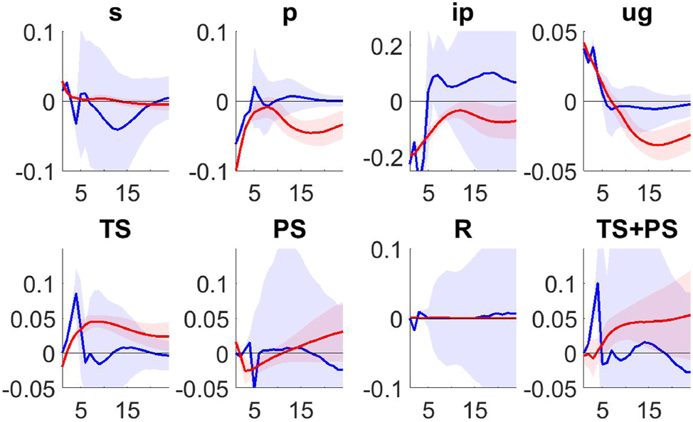
Figure 4 shows the responses from the VSTAR under the optimal policy rules (blue) to a credit shock during the ZLB period. For comparison, the corresponding responses from the estimated VSTAR, which reflect the dynamics under the actual Fed monetary policy are also reported (red).[33] According to these results, when the federal funds rate is constrained by the ZLB, the Fed responds under the optimal policy to a credit shock by increasing the size of the balance sheet more sharply than under the actual policy, at least in the short run (first 3 months). At the same time there is significant portfolio rebalancing towards Treasury securities, since TS holdings increase while PS holdings decrease in the short run horizon. The response of the Fed’s asset portfolio under the optimal policy show less persistence than those from the actual policy. This is because the optimal policy dampens very rapidly the impact of the shock on inflation and unemployment.
To illustrate how the optimal policy changes in response to different macroeconomic conditions, Figure 5 shows the responses under the actual (red) and optimal (blue) policy to a supply-type shock during the ZLB.[34] The federal funds rate remains constrained by the ZLB under both policies. The responses of QE are however different, being expansionary under the actual policy and contractionary under the optimal. The optimal QE policy response to the supply-type shock shows little rebalancing of the Fed portfolio contrary to what is observed from the responses to the credit shock displayed above.
In summary, QE under the optimal policy results in increase of the size of the balance sheet and significant short-run portfolio rebalancing toward TS in response to a credit-type shock. The responses to the supply-type shock are expansionary under the actual policy and contractionary under the optimal, with little evidence of portfolio rebalancing.
5.3 Counterfactual Monetary Policy
What would have been the dynamics of the economy and policy instruments had the federal funds rate and QE been coordinated optimally since 2008? To answer this question, the VSTAR under the optimal policy is used for three counterfactual experiments. The simulations are carried out starting from November 2007, using the specification of the Fed preferences with equal weights.
Each counterfactual simulation employs a different value for the inflation target, 2, 3 and 4 %. These do not reflect any specific view on the actual preferences of the Fed, but are selected for gauging indication on the sensitivity of the results to the choice of the inflation target.[35] It is important to clarify the role of the inflation target in these simulations. All other things equal, the optimal policy would require expansionary (contractionary) QE whenever actual inflation is below (above) target. As the unemployment gap is positive during most of the post-2007 period, the response of monetary policy to unemployment stabilization is stronger the lower is actual inflation relative to the target.
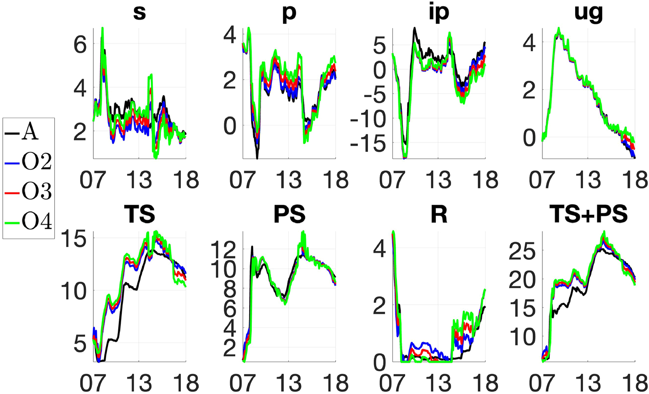
Figure 6 illustrates the results from these counterfactuals. Black lines (A) show the actual policy instruments dynamics as observed from data; whereas blue (O2), red (O3) and green (O4) lines denote the dynamics of the same instruments simulated from the optimal VSTAR under the three alternative inflation targets of 2, 3 and 4 %, respectively. The simulations are carried out assuming that in each period the Fed implements the optimal policy given the observed state of the economy.
Three main results can be observed from Figure 6. First, the dynamics of the economy are fairly similar across the three counterfactual simulations. Compared to the data, the main differences are that credit risk would have been lower and inflation higher during 2008–2013 under the optimal policy regardless of the choice of the inflation target. The dynamics of industrial production and the unemployment gap are remarkably similar to those observed from the data, under any of the three counterfactual simulations. Second, the path of the federal funds rate appears close to that observed from the data under any of the counterfactual simulations, particularly when using the 4 % inflation target. Third, the dynamics of the Fed’s balance sheet are qualitatively similar to the observed ones under any of the three counterfactual scenarios. The most noticeable exception is the period 2009–2015 period, when the size of the simulated Fed’s balance sheet is larger than the actual one. This is due to the more rapid increase in TS purchases under any of the counterfactual relative to the observed purchases.
Table 2 gives a breakdown of the duration of the ZLB period under the actual and optimal policy, based on the counterfactual analysis. In the data, the federal funds rate never reaches zero and the identification of the periods in which the ZLB is binding is somewhat arbitrary, depending on the chosen threshold below which the policy rate is deemed to be at the ZLB. To guard against this, the number of ZLB periods in Table 2 is counted considering four different thresholds, corresponding to months in which the federal funds rate is below to either 25, 50, 75 or 100 basis points. According to the results in the table, the actual duration of the ZLB ranges between 85 and 104 months, depending on the selected interest rate threshold. The duration of the ZLB from the counterfactual experiments is closer to the observed duration as the inflation target and the cut-off rate for the ZLB increase. It is worth highlighting that the estimated duration of the ZLB period is considerably longer than that otherwise predicted by conventional evaluations of monetary policy. For example, Williamson (2015) estimates that the ZLB should have terminated around the beginning of 2011 (26 months) had monetary policy during the Great Recession being conducted according to a standard Taylor rule.
The counterfactual simulations can be used to evaluate different segments of the QE intervention undertaken by the Fed since November 2007. The Fed embarked in three large-scale asset purchase programs, commonly known as QE1, QE2, QE3 and the Maturity Extension Program (MEP).[36] Table 3 reports how TS holding, PS holding and the total size of the Fed’s balance sheet change during each of these programs under the actual policy and the three counterfactual simulations. Under the actual QE policy, the total increase in the balance sheet was about 17.96 % of GDP. The size of the change of the Fed’s balance sheet as a percentage of GDP under the optimal policy is close to the actual one, ranging between 17.98 and 19.33 % depending on the inflation target. Comparing across programs, QE1 should have been almost a third larger, regardless of the inflation target. Consequently, this would have resulted in QE2 and QE3 programs of smaller size under the optimal policy compared to the actual. It would have also resulted in a reduction of the size of the balance sheet (relative to GDP) during the MEP under the optimal policy about four times larger than the actual reduction observed in the data.
Change in the Fed’s asset portfolio in percentage of GDP under actual and optimal policy over different QE phases.
| QE1 | QE2 | MEP | QE3 | Total | QE1 | QE2 | MEP | QE3 | Total | |
|---|---|---|---|---|---|---|---|---|---|---|
| Actual policy | Optimal policy,
|
|||||||||
| TS | 2.02 | 5.10 | −0.48 | 3.69 | 4.04 | 3.52 | −0.66 | 1.37 | ||
| PS | 5.35 | −1.75 | −0.08 | 4.12 | 7.37 | −1.83 | −1.51 | 5.68 | ||
| Total | 7.37 | 3.35 | −0.56 | 7.81 | 17.96 | 11.42 | 1.68 | −2.16 | 7.04 | 17.98 |
| Optimal policy,
|
Optimal policy,
|
|||||||||
| TS | 3.97 | 3.54 | −0.71 | 0.96 | 3.89 | 3.56 | −0.76 | 0.55 | ||
| PS | 8.06 | −1.82 | −1.63 | 6.30 | 8.74 | −1.81 | −1.76 | 6.92 | ||
| Total | 12.02 | 1.72 | −2.34 | 7.26 | 18.66 | 12.63 | 1.76 | −2.52 | 7.47 | 19.33 |
-
Source: Author’s calculations. See main text for more details.
As noted above, the counterfactual simulations under the optimal policy entail only small changes from the actual data. To provide some indication of the extent of these small changes, Table 4 reports in the top row the mean of the absolute deviation from the actual data of the macroeconomic forecasts from the Survey of Professional Forecasters of the Federal Reserve Bank of Philadelphia during 2007:11-2018:10, whereas the remaining rows report the corresponding deviations for the simulated data used for the results in Figure 6 and Table 1.[37] The table does not include TS and PS since the Survey covers all macroeconomic data used in the empirical analysis except for the balance sheet. The results in Table 4 provide some reassurance with regard to the closeness of the simulated data to the actual data. The counterfactual simulations involve smaller deviations from the actual data compared to the professional forecasts, for inflation, industrial production and unemployment, whereas the deviations for the spread the federal funds rate are marginally larger.
Mean of the absolute deviation from actual data of professional forecasts and simulated data from optimal policy, November 2007 – October 2018.
| s | p | ip | ug | R | |
|---|---|---|---|---|---|
| Professional forecasts | |||||
| 0.178 | 0.680 | 2.752 | 0.123 | 0.117 | |
| Optimal policy | |||||
|
|
0.590 | 0.180 | 1.785 | 0.048 | 0.323 |
|
|
0.562 | 0.356 | 2.108 | 0.083 | 0.313 |
|
|
0.592 | 0.604 | 2.447 | 0.139 | 0.377 |
| 1.55 | |||||
| (Baseline) | 0.630 | 0.163 | 1.785 | 0.046 | 0.359 |
| (Weights II) | 0.673 | 0.164 | 1.813 | 0.048 | 0.380 |
| (Weights III) | 0.442 | 0.162 | 1.292 | 0.038 | 0.288 |
| (Weights VI) | 0.844 | 0.191 | 2.401 | 0.058 | 0.449 |
| (Weights V) | 0.777 | 0.164 | 2.276 | 0.052 | 0.364 |
| (Weights VI) | 0.686 | 0.200 | 1.893 | 0.052 | 0.446 |
-
Source: Author’s calculations. See main text for more details.
In summary, according to this analysis the scale of total QE intervention observed in the data appears to be close to that prescribed by the optimal QE policy under conventional calibration of the Fed preferences. The main differences between actual and optimal QE are in terms of timing and composition, since the optimal QE would have entailed earlier increases in the Fed’s holding of TS compared to the actual policy. This would have resulted in lower spread and higher inflation in the aftermath of the Great Recession. Overall the counterfactual simulations indicate that the observed duration of the ZLB is in line with that otherwise prescribed by the optimal policy under most calibrations.
5.4 Alternative Optimization
The results presented above are the outcomes of two important requirements of the proposed optimization methodology: transformation of the VSTAR into a VSTARX using A2 and optimization with the SDC method. To evaluate the performance of the proposed optimization methodology, the results are compared with those from three possible alter- native approaches.[38] The first, labelled as LIN, is based on the linearized-equivalent of the VSTAR, i.e. the VAR model estimated over the same sample period, whose performance against the VSTAR is highlighted in Appendix E in Supplementary Material. As it is a reduced-form model, for the purpose of this exercise the VAR is transformed into a VARX using A2. The optimization problem then boils down to a LQR which is solved with standard Riccati equation iteration. The second and third approach both employ the VSTARX obtained from the estimated VSTAR under A1. For this reason optimization can only be undertaken with nonlinear methods. In the second, labelled as MPC, this is pursued using a method that mimics the logic of the model predictive control algorithm, whose application in a number of nonlinear decision problems in economics has been recently illustrated by Grüne et al. (2015). This consists of positing a time-varying coefficients feedback rule
Table 5 gives a summary of the outcomes of these numerical experiments, considering optimization for the post-2007 period and the full sample. For each approach and sample, the optimization is carried using the protocol and each of the six weight specifications described in Section 5.1. The first eighth columns of Table 5 report the average across all specifications of each argument in the loss function (15), the value of the loss V, the stabilization gain G and the unemployment-equivalent compensation
Average gains under alternative optimization methods.
|
|
|
|
|
|
V | G |
|
Speed (sec.) | |
|---|---|---|---|---|---|---|---|---|---|
| Sample: 2008:8–2018:9 | |||||||||
| Actual policy | 1.24 | 5.46 | 0.02 | 0.05 | 0.38 | 6.51 | |||
| Optimal policy | |||||||||
| SDC | 1.03 | 5.32 | 0.06 | 0.28 | 0.41 | 6.40 | 1.71 | 0.33 | 0.494 |
| LIN | 1.02 | 5.10 | 0.05 | 0.05 | 0.32 | 5.93 | 8.94 | 0.80 | 0.503 |
| MPC | 1.14 | 5.44 | 0.08 | 0.05 | 0.38 | 6.45 | 0.93 | 0.25 | 6.580 |
| DNS | 1.14 | 5.44 | 0.08 | 0.05 | 0.38 | 6.45 | 1.01 | 0.27 | 4.399 |
| Sample: 1979:8–2018:9 | |||||||||
| Actual policy | 4.75 | 2.66 | 0.32 | 0.02 | 0.11 | 7.16 | |||
| Optimal policy | |||||||||
| SDC | 3.40 | 2.38 | 0.36 | 0.14 | 0.20 | 5.82 | 18.42 | 1.22 | 1.539 |
| LIN | 3.91 | 2.48 | 0.31 | 0.02 | 0.19 | 6.24 | 12.58 | 1.01 | 1.768 |
| MPC | 4.62 | 2.64 | 0.30 | 0.02 | 0.11 | 7.01 | 2.06 | 0.41 | 21.592 |
| DNS | 4.62 | 2.64 | 0.46 | 0.02 | 0.11 | 7.14 | 0.365 | 0.12 | 15.351 |
-
Source: Author’s calculations. See main text for more details.
According to the results in Table 5, each optimization approach can deliver a feasible solution, i.e. a solution that leads to a loss lower than under the actual policy. Regarding efficiency, the results from these numerical experiments suggest that SDC and LIN provide superior performance compared to the two numerical methods, as indicated from the lower losses (and therefore stabilization gains and unemployment compensations) that these two approaches deliver regardless of the sample choice. The comparison between SDC and LIN needs careful interpretation. This is because the analysis of optimal policy with LIN is based on the linear VAR model, which gives a very poor fit of the data dynamics compared to the VSTAR which is used by SDC, as shown in Appendix in Supplementary Material, Table E.2. Further, the performance of LIN relative to SDC deteriorates as the simulation horizon is extended to cover the whole sample, thereby exacerbating the importance of nonliterary in the data. This points towards the importance of accounting for nonlinearity in the quantitative analysis of monetary policy, highlighting the difference it makes using a VAR rather than a nonlinear model like the VSTAR. Finally, optimization with SDC and LIN is way much faster than with the two numerical methods. This is not surprising since iteration until convergence of the Riccati equation in SDC and LIN is known to be faster than numerical search.
6 Conclusions
Macroeconomic data display many nonlinear features (asymmetries, thresholds and large swings) that often make linear models inadequate for reliable quantitative analysis. VSTAR is a popular tool employed in econometrics and applied macroeconomics for inference, structural analysis and forecasting when data are nonlinear. This paper uses VSTAR for a different task, the analysis of optimal policy.
At least two possible VSTARX can be employed to calculate optimal policy from a reduced-form VSTAR. One of these makes the analysis particularly tractable, since it preserves certainty equivalence and ensures low dimensionality of the decision making problem. The optimization employs SDC factorization to transform the VSTARX into a VAR with SDC matrices. This makes the NLQR problem isomorphic the LQR. Consequently, a nonlinear optimization problem can be solved with the same dynamic programming techniques used for LQR.
The methodology is applied to revisit the coordination between interest rate monetary policy and QE in the United States since 2008 and evaluate its effects on wider economy. To this end, the empirical analysis first establishes an estimated VSTAR that can be regarded as a reliable starting point for the subsequent policy analysis. According to the results found in the empirical analysis, the quantity of assets purchased the Fed and the duration of the ZLB in the decade after the onset of the Great Recession are not too dissimilar from those otherwise prescribed by the optimal policy. While the ZLB duration prescribed under the optimal policy is in line with the actual duration, there are however differences in terms of the timing and composition of QE. It is shown that the proposed methodology compares favourably, in terms of feasibility, efficiency and computational speed, with three alternative optimization approaches based on linear and nonlinear methods.
References
Atanasova, C. 2003. “Credit Market Imperfections and Business Cycle Dynamics: A Nonlinear Approach.” Studies in Nonlinear Dynamics & Econometrics 7 (4). https://doi.org/10.2202/1558-3708.1112.Suche in Google Scholar
Auerbach, A. J., and Y. Gorodnichenko. 2012. “Measuring the Output Responses to Fiscal Policy.” American Economic Journal: Economic Policy 4 (2): 1–27. https://doi.org/10.1257/pol.4.2.1.Suche in Google Scholar
Ball, L. M. 2014. The Case for a Long-run Inflation Target of Four Percent. IMF Working Papers 2014, 092. Washington, D.C.: International Monetary Fund.10.5089/9781498395601.001Suche in Google Scholar
Barnichon, R., and G. Mesters. 2023. “A Sufficient Statistics Approach for Macro Policy.” American Economic Review 113 (11): 2809–45. https://doi.org/10.1257/aer.20220581.Suche in Google Scholar
Beeler, S. C., H. T. Tran, and H. T. Banks. 2000. “Feedback Control Methodologies for Nonlinear Systems.” Journal of Optimization Theory and Applications 107 (1): 1–33. https://doi.org/10.1023/a:1004607114958.10.1023/A:1004607114958Suche in Google Scholar
Beraja, M. 2023. “A Semistructural Methodology for Policy Counterfactuals.” Journal of Political Economy 131 (1): 190–201. https://doi.org/10.1086/720982.Suche in Google Scholar
Chari, V. V., P. J. Kehoe, and E. R. McGrattan. 2009. “New Keynesian Models: Not yet Useful for Policy Analysis.” American Economic Journal: Macroeconomics 1 (1): 242–66. https://doi.org/10.1257/mac.1.1.242.Suche in Google Scholar
Dahlhaus, T. 2017. “Conventional Monetary Policy Transmission During Financial Crises: An Empirical Analysis.” Journal of Applied Econometrics 32 (2): 401–21. https://doi.org/10.1002/jae.2524.Suche in Google Scholar
Dahlhaus, T., K. Hess, and A. Reza. 2018. “International Transmission Channels of US Quantitative Easing: Evidence from Canada.” Journal of Money, Credit and Banking 50 (2-3): 545–63. https://doi.org/10.1111/jmcb.12470.Suche in Google Scholar
Del Negro, M., G. Eggertsson, A. Ferrero, and N. Kiyotaki. 2017. “The Great Escape? A Quantitative Evaluation of the Fed’s Liquidity Facilities.” American Economic Review 107 (3): 824–57. https://doi.org/10.1257/aer.20121660.Suche in Google Scholar
Dennis, R., and U. Söderström. 2006. “How Important is Precommitment for Monetary Policy?” Journal of Money, Credit and Banking: 847–72. https://doi.org/10.1353/mcb.2006.0054.Suche in Google Scholar
Dijk, D. V., T. Teräsvirta, and P. H. Franses. 2002. “Smooth Transition Autoregressive Models - A Survey of Recent Developments.” Econometric Reviews 21 (1): 1–47. https://doi.org/10.1081/etc-120002918.Suche in Google Scholar
Galvão, A. B., and M. T. Owyang. 2018. “Financial Stress Regimes and the Macroeconomy.” Journal of Money, Credit and Banking 50 (7): 1479–505. https://doi.org/10.1111/jmcb.12491.Suche in Google Scholar
Gambacorta, L., B. Hofmann, and G. Peersman. 2014. “The Effectiveness of Unconventional Monetary Policy at the Zero Lower Bound: A Cross-Country Analysis.” Journal of Money, Credit and Banking 46 (4): 615–42. https://doi.org/10.1111/jmcb.12119.Suche in Google Scholar
Gefang, D., and R. Strachan. 2009. “Nonlinear Impacts of International Business Cycles on the UK - a Bayesian Smooth Transition VAR Approach.” Studies in Nonlinear Dynamics & Econometrics 14 (1). https://doi.org/10.2202/1558-3708.1677.Suche in Google Scholar
Granger, C. W., and T. Terasvirta. 1993. Modelling Non-Linear Economic Relationships. Oxford, UK: Oxford University Press.Suche in Google Scholar
Grüne, L., W. Semmler, and M. Stieler. 2015. “Using Nonlinear Model Predictive Control for Dynamic Decision Problems in Economics.” Journal of Economic Dynamics and Control 60: 112–33. https://doi.org/10.1016/j.jedc.2015.08.010.Suche in Google Scholar
Guerrieri, L., and M. Iacoviello. 2017. “Collateral Constraints and Macroeconomic Asymmetries.” Journal of Monetary Economics 90: 28–49. https://doi.org/10.1016/j.jmoneco.2017.06.004.Suche in Google Scholar
Hurn, S., N. Johnson, A. Silvennoinen, and T. Teräsvirta. 2022. “Transition from the Taylor Rule to the Zero Lower Bound.” Studies in Nonlinear Dynamics & Econometrics 26 (5): 635–47. https://doi.org/10.1515/snde-2019-0102.Suche in Google Scholar
Joyce, M., D. Miles, A. Scott, and D. Vayanos. 2012. “Quantitative Easing and Unconventional Monetary Policy - an Introduction.” The Economic Journal 122 (564): F271–88. https://doi.org/10.1111/j.1468-0297.2012.02551.x.Suche in Google Scholar
Kaiser, E., J. N. Kutz, and S. L. Brunton. 2017. “Data-Driven Discovery of Koopman Eigenfunctions for Control.” arXiv preprint arXiv:1707.01146.Suche in Google Scholar
Kapetanios, G., H. Mumtaz, I. Stevens, and K. Theodoridis. 2012. “Assessing the Economy-Wide Effects of Quantitative Easing.” The Economic Journal 122 (564): F316–47. https://doi.org/10.1111/j.1468-0297.2012.02555.x.Suche in Google Scholar
Koop, G., M. H. Pesaran, and S. M. Potter. 1996. “Impulse Response Analysis in Nonlinear Multivariate Models.” Journal of Econometrics 74 (1): 119–47. https://doi.org/10.1016/0304-4076(95)01753-4.Suche in Google Scholar
Kuttner, K. N. 2018. “Outside the Box: Unconventional Monetary Policy in the Great Recession and Beyond.” Journal of Economic Perspectives 32 (4): 121–46. https://doi.org/10.1257/jep.32.4.121.Suche in Google Scholar
Lanne, M., and P. Saikkonen. 2005. “Non-Linear GARCH Models for Highly Persistent Volatility.” The Econometrics Journal 8 (2): 251–76. https://doi.org/10.1111/j.1368-423x.2005.00163.x.Suche in Google Scholar
Lenza, M., H. Pill, and L. Reichlin. 2010. “Monetary Policy in Exceptional Times.” Economic Policy 25 (62): 295–339. https://doi.org/10.1111/j.1468-0327.2010.00240.x.Suche in Google Scholar
Liu, P., K. Theodoridis, H. Mumtaz, and F. Zanetti. 2019. “Changing Macroeconomic Dynamics at the Zero Lower Bound.” Journal of Business & Economic Statistics 37 (3): 391–404. https://doi.org/10.1080/07350015.2017.1350186.Suche in Google Scholar
Ljungqvist, L., and T. J. Sargent. 2018. Recursive Macroeconomic Theory. Cambridge, Massachusetts: MIT press.Suche in Google Scholar
Lucas, R. E. 1976. “Econometric Policy Evaluation: A Critique.” In Carnegie-Rochester Conference Series on Public Policy, Vol. 1, 19–46. North-Holland. https://www.sciencedirect.com/science/article/pii/S0167223176800036.10.1016/S0167-2231(76)80003-6Suche in Google Scholar
Luukkonen, R., P. Saikkonen, and T. Teräsvirta. 1988. “Testing Linearity Against Smooth Transition Autoregressive Models.” Biometrika 75 (3): 491–9. https://doi.org/10.1093/biomet/75.3.491.Suche in Google Scholar
Martin, V., S. Hurn, and D. Harris. 2013. Econometric Modelling with Time Series: Specification, Estimation and Testing. Cambridge, UK: Cambridge University Press.10.1017/CBO9781139043205Suche in Google Scholar
McKay, A., and C. K. Wolf. 2023. “What Can time-series Regressions Tell us About Policy Counterfactuals?” Econometrica 91 (5): 1695–725. https://doi.org/10.3982/ecta21045.Suche in Google Scholar
Pearson, J. 1962. “Approximation Methods in Optimal Control I. Sub-Optimal Control.” International Journal of Electronics 13 (5): 453–69. https://doi.org/10.1080/00207216208937454.Suche in Google Scholar
Polito, V., and P. Spencer. 2016. “Optimal Control of Heteroscedastic Macroeconomic Models.” Journal of Applied Econometrics 31 (7): 1430–44. https://doi.org/10.1002/jae.2488.Suche in Google Scholar
Polito, V., and M. Wickens. 2012. “Optimal Monetary Policy Using an Unrestricted VAR.” Journal of Applied Econometrics 27 (4): 525–53. https://doi.org/10.1002/jae.1219.Suche in Google Scholar
Ramey, V. A., and S. Zubairy. 2018. “Government Spending Multipliers in Good Times and in Bad: Evidence from US Historical Data.” Journal of Political Economy 126 (2): 850–901. https://doi.org/10.1086/696277.Suche in Google Scholar
Rudebusch, G. D. 2005. “Assessing the Lucas Critique in Monetary Policy Models.” Journal of Money, Credit and Banking 37 (2): 245–72, https://doi.org/10.1353/mcb.2005.0024.Suche in Google Scholar
Sack, B. 2000. “Does the Fed Act Gradually? A VAR Analysis.” Journal of Monetary Economics 46 (1): 229–56. https://doi.org/10.1016/s0304-3932(00)00019-2.Suche in Google Scholar
Sims, E. R., and J. C. Wu. 2020. “Are QE and Conventional Monetary Policy Substitutable?” International Journal of Central Banking 16 (1): 195–230.Suche in Google Scholar
Sims, E., and J. C. Wu. 2021. “Evaluating Central Banks’ Tool Kit: Past, Present, and Future.” Journal of Monetary Economics 118: 135–60. https://doi.org/10.1016/j.jmoneco.2020.03.018.Suche in Google Scholar
Sims, C. A., and T. Zha. 2006. “Were There Regime Switches in US Monetary Policy?” American Economic Review 96 (1): 54–81. https://doi.org/10.1257/000282806776157678.Suche in Google Scholar
Sims, E., J. C. Wu, and J. Zhang. 2023. “The Four-Equation New Keynesian Model.” Review of Economics and Statistics 105 (4): 931–47. https://doi.org/10.1162/rest_a_01071.Suche in Google Scholar
Smets, F., and R. Wouters. 2003. “An Estimated Dynamic Stochastic General Equilibrium Model of the Euro Area.” Journal of the European Economic Association 1 (5): 1123–75. https://doi.org/10.1162/154247603770383415.Suche in Google Scholar
Stock, J. H., and M. W. Watson. 2001. “Vector Autoregressions.” Journal of Economic Perspectives 15 (4): 101–15. https://doi.org/10.1257/jep.15.4.101.Suche in Google Scholar
Terasvirta, T., and H. M. Anderson. 1992. “Characterizing Nonlinearities in Business Cycles Using Smooth Transition Autoregressive Models.” Journal of Applied Econometrics 7 (S1): S119–S136. https://doi.org/10.1002/jae.3950070509.Suche in Google Scholar
Wernli, A., and G. Cook. 1975. “Suboptimal Control for the Nonlinear Quadratic Regulator Problem.” Automatica 11 (1): 75–84. https://doi.org/10.1016/0005-1098(75)90010-2.Suche in Google Scholar
Williamson, S. 2015. “The Road to Normal: New Directions in Monetary Policy.” Annual Report: 6–23.Suche in Google Scholar
Supplementary Material
This article contains supplementary material (https://doi.org/10.1515/snde-2024-0100).
© 2025 the author(s), published by De Gruyter, Berlin/Boston
This work is licensed under the Creative Commons Attribution 4.0 International License.