Matrix autoregressive models: generalization and Bayesian estimation

Alessandro Celani; Paolo Pagnottoni

doi:10.1515/snde-2022-0093

Artikel

Matrix autoregressive models: generalization and Bayesian estimation

Alessandro Celani und Paolo Pagnottoni

Veröffentlicht/Copyright: 4. Juli 2023

Veröffentlicht von

Veröffentlichen auch Sie bei De Gruyter Brill

Manuskript einreichen Informationen für Autor*innen

Aus der Zeitschrift Studies in Nonlinear Dynamics & Econometrics Band 28 Heft 2

Abstract

The issue of modelling observations generated in matrix form over time is key in economics, finance and many domains of application. While it is common to model vectors of observations through standard vector time series analysis, original matrix-valued data often reflect different types of structures of time series observations which can be further exploited to model interdependencies. In this paper, we propose a novel matrix autoregressive model in a bilinear form which, while leading to a substantial dimensionality reduction and enhanced interpretability: (a) allows responses and potential covariates of interest to have different dimensions; (b) provides a suitable estimation procedure for matrix autoregression with lag structure; (c) facilitates the introduction of Bayesian estimators. We propose maximum likelihood and Bayesian estimation with Independent-Normal prior formulation, and study the theoretical properties of the estimators through simulated and real examples.

Keywords: autoregressive models; Bayesian estimation; bilinear autoregression; matrix-valued time series; multivariate time series; nearest Kronecker product projection

JEL Classification: C32; C33; C51; C11

Corresponding author: Alessandro Celani, School of Statistics, University of Minnesota Twin Cities, Minneapolis, USA; and Department of Economics and Social Sciences, Università Politecnica delle Marche, Ancona, Italy, E-mail: a.celani@pm.univpm.it

Funding source: Horizon 2020 Framework Programme

Award Identifier / Grant number: 101016233

Acknowledgment

The authors gratefully acknowledges the European Union’s Horizon 2020 research and innovation program “PERISCOPE: Pan European Response to the ImpactS of COVID-19 and future Pandemics and Epidemics”, under the grant agreement No. 101016233, H2020-SC1-PHE-CORONAVIRUS-2020-2-RTD.

Author contributions: All the authors have accepted responsibility for the entire content of this submitted manuscript and approved submission.
Research funding: None declared.
Conflict of interest statement: The authors declare no conflicts of interest regarding this article.

Appendix A: Tensor operations and the Tucker product

A tensor is a multidimensional array, whose order expresses the number of dimensions, also known as ways or modes.^[4] More formally, an Nth way tensor is an N dimensional array X ∈ R I 1 × ⋯ × I N with entries X i 1 … i N with i _n = 1, …, I _n and n = 1, …, N.

Vectors are tensors of order one (denoted by boldface lowercase letters, e.g., x) whereas matrices are tensors of order two (denoted by boldface capital letters, e.g., X).

A.1 Tensor norm and inner product

The Frobenius norm of a tensor X is the square root of the squared sum of all its elements, i.e.

‖ X ‖ F = ∑ j 1 = 1 J 1 … ∑ j N = 1 J N x j 1 … j N 2 = vec ( X ) ′ vec ( X )

which is analogous to the Frobenious norm of a matrix.

The inner-product of two tensors of the same dimension X , Y ∈ R J 1 , … , J N is the sum of the product of their entries:

⟨ X , Y ⟩ = ∑ j 1 = 1 J N … . ∑ j N = 1 J N x j 1 … j N y j 1 … j N = vec ( X ) ′ vec ( Y )

A.2 Matricization and Tucker product

The process of reordering the elements of an N-way array into a matrix is called matricization. The nth way matricization of X is denoted by X n = mat k ( X ) , and is obtained by reshaping the elements of the original tensor so that the resulting matrix is of dimension [I _n × ∏_j≠n I _j]. The special case of contemporaneous matricization along all the ways of a tensor is called vectorization, which is analogous to the vectorization of a matrix:

x = vec ( X ) = mat 1 , … , N ( X ) .

Given the matrices B ₁, …, B _N with B n ∈ R i n × j n , a map from the space of X to the space generated by the rows of B _n R i 1 × ⋯ × i N is made by first obtaining x, then computing:

m = ( B N ⊗ … . ⊗ B 1 ) x

and eventually forming an [i ₁× … ×i _N] dimensional array M from M. This transformation between the tensor X and the list B = {B ₁, …, B _N} is known as the Tucker product (Tucker 1966), and can be written as:

(25) M = X × ̄ { B 1 , … B N }

It is worth noting that the matricization operator connects the multidimensional Tucker product to the well known matrix multiplication, facilitating both understanding and computation of the former. In fact, by applying the nth way matricization to both sides of Equation (25) we obtain the equivalent formulation:

(26) M n = B n X n B − n ′

where B _−n = (B _N ⊗ … ⊗ B _n+1 ⊗ B _n−1 ⊗ … ⊗ B ₁). By repeating the operation for n = 1, …, N, it emerges that the Tucker product can be expressed as a series of N matrix reshaping and multiplications. Matricization and vectorization applied to the Tucker product give raise to the following set of equivalences:

M = X × ̄ { B 1 , … , B N } M n = B n X n B − n ′ = ( B N ⊗ … . ⊗ B 1 ) x .

The VAR as well as the MAR equivalent form of a TAR can be easily derived with the abovementioned tools.

Appendix B: Competing models

The PVAR in Equation (1) can be written in compact form as:

(27) Y = B X + E

where Y = [y _P+1, …, y _T] and the coefficient matrix B = [Φ ₁, …, Φ _P] is of dimension GN × GNP. X = [X _P, …, X _T−1] where X _t = [y _t−1, …, y _t−P]. We consider the following competing models:

CC: Canova and Ciccarelli (2009, 2013) use a factorization approach of the parameters such that they can be divided into common, country-specific, and variable-specific factors. They specify the model in a hierarchical structure:
(28) vec ( B ) | F ∼ N ( Λ F , Σ ⊗ I G N ) F ∼ N ( 0 , c ̲ F )
where Λ is an GN × f matrix of loadings and F is an f × 1 vector of factors where f < GN. Under this formulation we have N common factors for coeffcients of each country and, analogously, G common factors for coefficients of each indicators. Regarding the variance hyperparameter, we fix it as c ̲ = 4 .
SSVS: George, Sun, and Ni (2008) specify a prior whereby each coefficient of B is drawn from a Mixture of two normal distribution, the former with a small variance aiming at shrink the coefficient towards 0 and the latter with a relatively large one. The higher the magnitude of B _ij the higher is the probability that it will be drawn from the second distribution, and viceversa.
(29) vec ( B ) k | γ k ∼ ( 1 − γ k ) N 0 , τ ̲ 1 2 + γ k N 0 , τ ̲ 2 2 γ k ∼ B e r ( π ̲ k )
with k = 1, …, G ² N ² P and where we set τ ̲ 1 2 = 0.01 , τ ̲ 2 2 = 4 and π ̲ k = 0.5 .
SSSS: This algorithm created by Koop and Korobilis (2016) builds on George, Sun, and Ni (2008) but takes in into account Panel restrictions. They specify three priors based on the possible restrictions: no dynamic interdependencies, no static interdependencies and for homogeneity across coefficient matrices.

The dynamic interdependency works on off-block diagonal blocks. Let B _ij ∈ B be the G × G block embodying parameters of country j on country i equations. The prior has the following form:
(30) B i j | γ i j D I ∼ 1 − γ i j D I N 0 , τ ̲ 1 2 I G + γ i j D I N 0 , τ ̲ 2 2 I G γ i j D I | π i j D I ∼ B e r π i j D I , ∀ j i π i j D I ∼ B e t a ( 1 , ϕ )
while the cross-sectional homogeneity prior is set on the main block diagonal of f B. The prior reads as:
(31) B i i | γ i j CSH ∼ 1 − γ i j CSH N B j j , ξ ̲ 1 2 I G + γ i j CSH N B j j , ξ ̲ 2 2 I G γ i j CSH | π i j CSH ∼ B e r π i j CSH , ∀ j ≠ i π i j CSH ∼ B e t a ( 1 , ϕ )
where we set τ ̲ 1 2 , ξ ̲ 1 2 = 0.01 , τ ̲ 2 2 , ξ ̲ 2 2 = 4 , π i j D I , π i j CSH = 0.5 and π ̲ k = 1 .
Lasso VAR: is a regression method suited for multivariate models such as the VAR that performs both variable selection and ℓ ₁ regularization enhancing the prediction accuracy and model interpretability Rothman, Levina, and Zhu (2010) and Schnücker (2019). It produces a sparse version of B which is solution to the following problem:
(32) B ̂ = arg min B ( Y − B X ) Σ − 1 ( Y − B X ) + ∑ i = 1 G N ∑ j = 1 G N λ i j | B i j |

We fix a basic penalty of λ _ij = 0.1 if B _ij belongs to country block diagonal elements of B and a more restrictive one of λ _ij = 0.5 if the parameter is related to the off-block diagonal ones.

Appendix C: Full conditional distribution of γ

Using a gamma prior distribution we have:

p γ | Σ 1 , Σ 2 , Σ 3 ∝ p Σ 1 , Σ 2 , Σ 3 | γ π ( γ ) ∝ ∏ i = 1 3 γ Ψ i − ν i 2 ⁡ exp − 1 2 t r γ Ψ i Σ i − 1 γ a γ − 1 ⁡ exp − b γ γ ∝ γ a γ − ∑ i = 1 3 ν i I i 2 − 1 ⁡ exp − 1 2 t r ∑ i = 1 3 Ψ i Σ i − 1 − b γ γ

thus:

p γ | Σ 1 , Σ 2 , Σ 3 ∼ G a a γ + 1 2 ∑ i = 1 3 ν i I i , b γ + 1 2 t r ∑ i = 1 3 Ψ i Σ i − 1

Appendix D: Additional application results

Table 2:

Median of the posterior distribution of C ₀ (a) and D ₀ (b).

	ARM	M	CO
(a)
IR	−0.006	−0.022	0.002
CPI	0.026	0.011	0.001
E/I	−0.090	−0.031	0.003
IP	0.017	−0.002	0.005
RT	0.064	0.032	0.006
UN	−0.146	−0.027	−0.020
(b)
CA	0.005	0.007	−0.022
FR	0.020	0.015	0.002
DE	−0.016	0.043	0.017
IT	0.031	−0.009	−0.001
JP	0.006	0.008	0.013
NL	0.015	−0.035	−0.006
ES	0.057	−0.018	−0.001
GB	0.024	0.027	0.015
US	−0.002	0.004	−0.010

Figure 8:

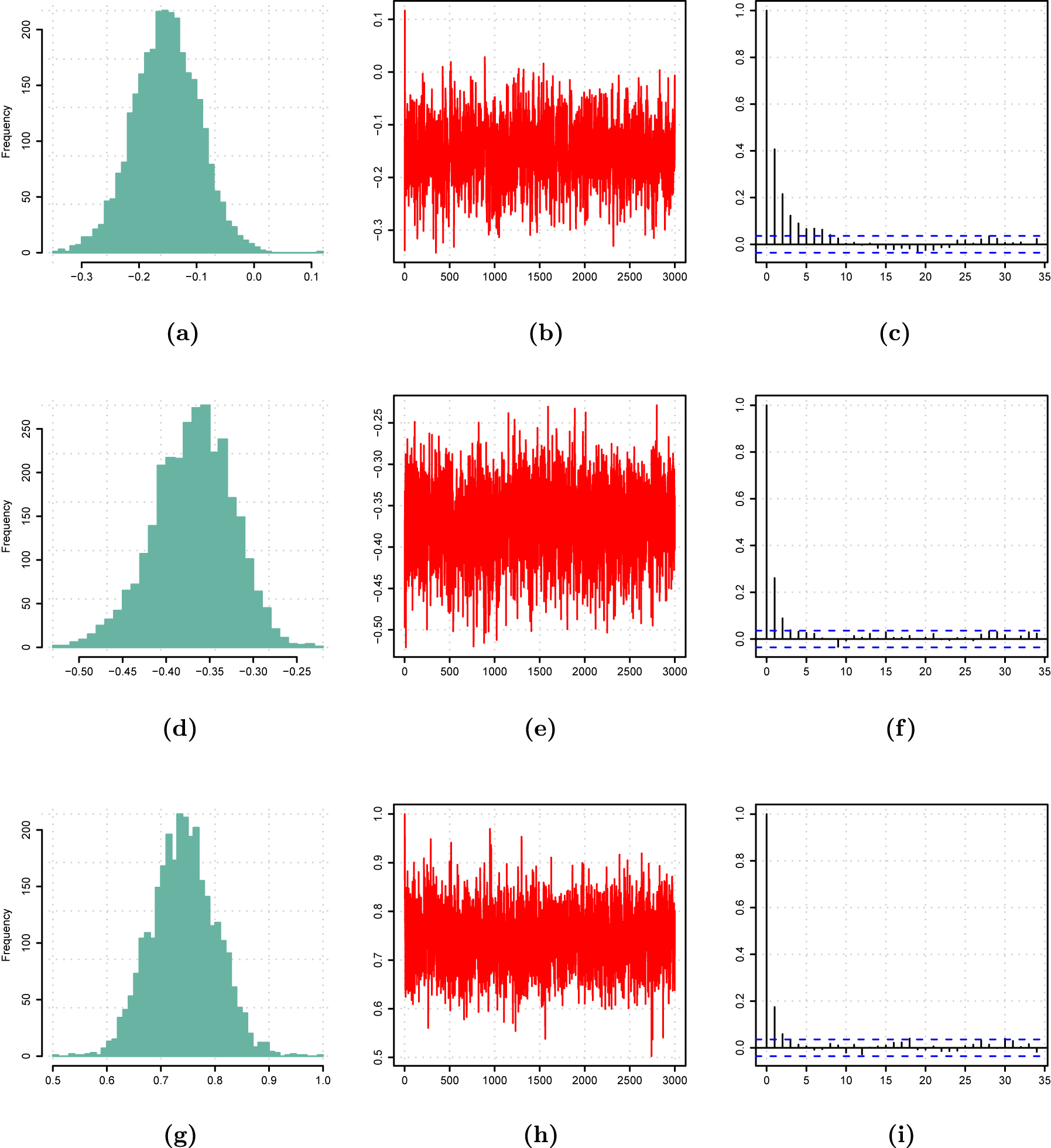
Posterior distribution (left), MCMC output (middle) and autocorrelation function (right) of three randomly selected entries of A ₁.

References

Ahelegbey, D., M. Billio, and R. Casarin. 2016a. “Bayesian Graphical Models for Structural Vector Autoregressive Processes.” Journal of Applied Econometrics 31 (2): 357–86. https://doi.org/10.1002/jae.2443.Suche in Google Scholar

Ahelegbey, D. F., M. Billio, and R. Casarin. 2016b. “Sparse Graphical Vector Autoregression: A Bayesian Approach.” Annals of Economics and Statistics (123/124): 333–61. https://doi.org/10.15609/annaeconstat2009.123-124.0333.Suche in Google Scholar

Bai, J., and S. Ng. 2002. “Determining the Number of Factors in Approximate Factor Models.” Econometrica 70 (1): 191–221. https://doi.org/10.1111/1468-0262.00273.Suche in Google Scholar

Bańbura, M., D. Giannone, and L. Reichlin. 2010. “Large Bayesian Vector Auto Regressions.” Journal of Applied Econometrics 25 (1): 71–92. https://doi.org/10.1002/jae.1137.Suche in Google Scholar

Billio, M., R. Casarin, M. Iacopini, and S. Kaufmann. 2023. “Bayesian Dynamic Tensor Regression.” Journal of Business & Economic Statistics 41 (2): 429–39, https://doi.org/10.1080/07350015.2022.2032721.Suche in Google Scholar

Brown, P., and J. Griffin. 2010. “Inference with Normal-Gamma Prior Distributions in Regression Problems.” Bayesian Analysis 5 (1): 171–88. https://doi.org/10.1214/10-ba507.Suche in Google Scholar

Canova, F., and M. Ciccarelli. 2009. “Estimating Multicountry Var Models.” International Economic Review 50 (3): 929–59. https://doi.org/10.1111/j.1468-2354.2009.00554.x.Suche in Google Scholar

Canova, F., and M. Ciccarelli. 2013. “Panel Vector Autoregressive Models: A Survey.” Advances in Econometrics 31: 205–46.10.1108/S0731-9053(2013)0000031006Suche in Google Scholar

Chen, R., H. Xiao, and D. Yang. 2021. “Autoregressive Models for Matrix-Valued Time Series.” Journal of Econometrics 222 (1): 539–60. https://doi.org/10.1016/j.jeconom.2020.07.015.Suche in Google Scholar

Comon, P. 2014. “Tensors: A Brief Introduction.” IEEE Signal Processing Magazine 31 (3): 44–53. https://doi.org/10.1109/msp.2014.2298533.Suche in Google Scholar

Czudaj, R. L. 2019. “Dynamics between Trading Volume, Volatility and Open Interest in Agricultural Futures Markets: A Bayesian Time-Varying Coefficient Approach.” Econometrics and Statistics 12: 78–145. https://doi.org/10.1016/j.ecosta.2019.05.002.Suche in Google Scholar

Durante, D., and D. B. Dunson. 2014. “Bayesian Dynamic Financial Networks with Time-Varying Predictors.” Statistics & Probability Letters 93: 19–26. https://doi.org/10.1016/j.spl.2014.06.015.Suche in Google Scholar

Filippeli, T., R. Harrison, and K. Theodoridis. 2020. “Dsge-based Priors for Bvars and Quasi-Bayesian Dsge Estimation.” Econometrics and Statistics 16: 1–27. https://doi.org/10.1016/j.ecosta.2018.12.002.Suche in Google Scholar

Follett, L., and C. Yu. 2019. “Achieving Parsimony in Bayesian Vector Autoregressions with the Horseshoe Prior.” Econometrics and Statistics 11: 130–44. https://doi.org/10.1016/j.ecosta.2018.12.004.Suche in Google Scholar

Forni, M., M. Hallin, M. Lippi, and L. Reichlin. 2005. “The Generalized Dynamic Factor Model.” Journal of the American Statistical Association 100 (471): 830–40. https://doi.org/10.1198/016214504000002050.Suche in Google Scholar

Gefang, D. 2014. “Bayesian Doubly Adaptive Elastic-Net Lasso for Var Shrinkage.” International Journal of Forecasting 30 (1): 1–11. https://doi.org/10.1016/j.ijforecast.2013.04.004.Suche in Google Scholar

George, E. I., D. Sun, and S. Ni. 2008. “Bayesian Stochastic Search for Var Model Restrictions.” Journal of Econometrics 142 (1): 553–80. https://doi.org/10.1016/j.jeconom.2007.08.017.Suche in Google Scholar

Gong, L., and J. M. Flegal. 2016. “A Practical Sequential Stopping Rule for High-Dimensional Markov Chain Monte Carlo.” Journal of Computational & Graphical Statistics 25 (3): 684–700. https://doi.org/10.1080/10618600.2015.1044092.Suche in Google Scholar

Gupta, A., and D. K. Nagar. 1999. Matrix Variate Distributions, 104. Boca Raton: CRC Press.Suche in Google Scholar

Hoff, P. D. 2015. “Multilinear Tensor Regression for Longitudinal Relational Data.” Annals of Applied Statistics 9 (3): 1169–93. https://doi.org/10.1214/15-aoas839.Suche in Google Scholar PubMed PubMed Central

Hung, H., and W. Chen-Chien. 2012. “Matrix Variate Logistic Regression Model with Application to EEG Data.” Biostatistics 14 (1): 189–202. https://doi.org/10.1093/biostatistics/kxs023.Suche in Google Scholar PubMed

Kock, A., and L. Callot. 2015. “Oracle Inequalities for High Dimensional Vector Autoregressions.” Journal of Econometrics 186 (2): 325–44. https://doi.org/10.1016/j.jeconom.2015.02.013.Suche in Google Scholar

Kolda, T. G., and B. W. Bader. 2009. “Tensor Decompositions and Applications.” SIAM Review 51 (3): 455–500. https://doi.org/10.1137/07070111x.Suche in Google Scholar

Koop, G., and D. Korobilis. 2016. “Model Uncertainty in Panel Vector Autoregressive Models.” European Economic Review 81: 115–31. https://doi.org/10.1016/j.euroecorev.2015.09.006.Suche in Google Scholar

Koop, G., M. Pesaran, and S. M. Potter. 1996. “Impulse Response Analysis in Nonlinear Multivariate Models.” Journal of Econometrics 74 (1): 119–47. https://doi.org/10.1016/0304-4076(95)01753-4.Suche in Google Scholar

Korobilis, D. 2016. “Prior Selection for Panel Vector Autoregressions.” Computational Statistics & Data Analysis 101: 110–20. https://doi.org/10.1016/j.csda.2016.02.011.Suche in Google Scholar

Korobilis, D. 2021. “High-Dimensional Macroeconomic Forecasting Using Message Passing Algorithms.” Journal of Business & Economic Statistics 39 (2): 493–504. https://doi.org/10.1080/07350015.2019.1677472.Suche in Google Scholar

Lai, W.-T., R.-B. Chen, Y. Chen, and T. Koch. 2022. “Variational Bayesian Inference for Network Autoregression Models.” Computational Statistics & Data Analysis 169: 107406. https://doi.org/10.1016/j.csda.2021.107406.Suche in Google Scholar

Lee, N., H. Choi, and S.-H. Kim. 2016. “Bayes Shrinkage Estimation for High-Dimensional Var Models with Scale Mixture of Normal Distributions for Noise.” Computational Statistics & Data Analysis 101: 250–76. https://doi.org/10.1016/j.csda.2016.03.007.Suche in Google Scholar

Li, L., and X. Zhang. 2017. “Parsimonious Tensor Response Regression.” Journal of the American Statistical Association 112 (519): 1131–46. https://doi.org/10.1080/01621459.2016.1193022.Suche in Google Scholar

Loperfido, N. 2017. “A New Kurtosis Matrix, with Statistical Applications.” Linear Algebra and its Applications 512: 1–17. https://doi.org/10.1016/j.laa.2016.09.033.Suche in Google Scholar

Loperfido, N. 2018. “Skewness-based Projection Pursuit: A Computational Approach.” Computational Statistics & Data Analysis 120: 42–57. https://doi.org/10.1016/j.csda.2017.11.001.Suche in Google Scholar

Loperfido, N. 2019. “Finite Mixtures, Projection Pursuit and Tensor Rank: A Triangulation.” Advances in Data Analysis and Classification 13 (1): 145–73. https://doi.org/10.1007/s11634-018-0336-z.Suche in Google Scholar

Lütkepohl, H. 2005. New Introduction to Multiple Time Series Analysis. Berlin: Springer.10.1007/978-3-540-27752-1Suche in Google Scholar

Nardi, Y., and A. Rinaldo. 2011. “Autoregressive Process Modeling via the Lasso Procedure.” Journal of Multivariate Analysis 102 (3): 528–49. https://doi.org/10.1016/j.jmva.2010.10.012.Suche in Google Scholar

Park, T., and G. Casella. 2008. “The Bayesian Lasso.” Journal of the American Statistical Association 103 (482): 681–6. https://doi.org/10.1198/016214508000000337.Suche in Google Scholar

Rothman, A. J., E. Levina, and J. Zhu. 2010. “Sparse Multivariate Regression with Covariance Estimation.” Journal of Computational & Graphical Statistics 19 (4): 947–62. https://doi.org/10.1198/jcgs.2010.09188.Suche in Google Scholar PubMed PubMed Central

Schnücker, A. 2019. “Penalized Estimation of Panel Vector Autoregressive Models.” Econometric Institute Research Papers EI-2019-33. Erasmus University Rotterdam, Erasmus School of Economics (ESE), Econometric Institute.Suche in Google Scholar

Song, S. and P. Bickel. 2011. “Large Vector Auto Regressions.” Papers, arXiv.org.Suche in Google Scholar

Tucker, L. R. 1966. “Some Mathematical Notes on Three-Mode Factor Analysis.” Psychometrika 51: 279–311. https://doi.org/10.1007/bf02289464.Suche in Google Scholar PubMed

Van Loan, C. F. 2000. “The Ubiquitous Kronecker Product.” Journal of Computational and Applied Mathematics 123 (1): 85–100. https://doi.org/10.1016/s0377-0427(00)00393-9.Suche in Google Scholar

Van Loan, C. F., and N. Pitsianis. 1993. Approximation with Kronecker Products, 293–314. Dordrecht: Springer Netherlands.10.1007/978-94-015-8196-7_17Suche in Google Scholar

Vats, D., J. M. Flegal, and G. L. Jones. 2019. “Multivariate Output Analysis for Markov Chain Monte Carlo.” Biometrika 106 (2): 321–37. https://doi.org/10.1093/biomet/asz002.Suche in Google Scholar

Wang, H., and M. West. 2009. “Bayesian Analysis of Matrix Normal Graphical Models.” Biometrika 96 (4): 821–34. https://doi.org/10.1093/biomet/asp049.Suche in Google Scholar PubMed PubMed Central

Wang, D., X. Liu, and R. Chen. 2019. “Factor Models for Matrix-Valued High-Dimensional Time Series.” Journal of Econometrics 208 (1): 231–48. https://doi.org/10.1016/j.jeconom.2018.09.013.Suche in Google Scholar

Zhao, Q., L. Zhang, and A. Cichocki. 2013. “A Tensor-Variate Gaussian Process for Classification of Multidimensional Structured Data.” Proceedings of the AAAI Conference on Artificial Intelligence 27 (1): 1041–7. https://doi.org/10.1609/aaai.v27i1.8568.Suche in Google Scholar

Zhou, H., L. Li, and H. Zhu. 2013. “Tensor Regression with Applications in Neuroimaging Data Analysis.” Journal of the American Statistical Association 108 (502): 540–52. https://doi.org/10.1080/01621459.2013.776499.Suche in Google Scholar PubMed PubMed Central

Received: 2022-10-14

Accepted: 2023-05-22

Published Online: 2023-07-04

Sie haben derzeit keinen Zugang zu diesem Inhalt.

Artikel in diesem Heft

https://doi.org/10.1515/snde-2022-0093

Schlagwörter für diesen Artikel

autoregressive models; Bayesian estimation; bilinear autoregression; matrix-valued time series; multivariate time series; nearest Kronecker product projection

Matrix autoregressive models: generalization and Bayesian estimation

Artikel

Abstract

Acknowledgment

Appendix A: Tensor operations and the Tucker product

A.1 Tensor norm and inner product

A.2 Matricization and Tucker product

Appendix B: Competing models

Appendix C: Full conditional distribution of γ

Appendix D: Additional application results

References

Artikel in diesem Heft

Artikel in diesem Heft

Artikel in diesem Heft

A.1 Tensor norm and inner product