Markov-Switching Models with Unknown Error Distributions: Identification and Inference Within the Bayesian Framework
-
Shih-Tang Hwu


Abstract
The basic Markov-switching model has been extended in various ways ever since the seminal work of Hamilton (1989. “A New Approach to the Economic Analysis of Nonstationary Time Series and the Business Cycle.” Econometrica 57: 357–84). However, the estimation of Markov-switching models in the literature has relied upon parametric assumptions on the distribution of the error term. In this paper, we present a Bayesian approach for estimating Markov-switching models with unknown and potentially non-normal error distributions. We approximate the unknown distribution of the error term by the Dirichlet process mixture of normals, in which the number of mixtures is treated as a parameter to estimate. In doing so, we pay special attention to the identification of the model. We then apply the proposed model and MCMC procedure to the growth of the postwar U.S. industrial production index. Our model can effectively control for irregular components that are not related to business conditions. This leads to sharp and accurate inferences on recession probabilities.
1 Introduction
Since the seminal work of Hamilton (1989), the basic Markov-switching model has been extended in various ways. For example, Diebold, Lee, and Weinbach (1994) and Filardo (1994) extend the model to allow the transition probabilities governing the Markov process to be functions of exogenous or predetermined variables. Kim (1994) extends it to the case of the state-space model, which encompasses general dynamic models such as autoregressive moving average processes, unobserved components models, dynamic factor models, etc. Chib (1998) introduces a structural break model with unknown multiple change points by constraining the transition probabilities of the Markov-switching model so that the latent state variable can either stay at the current value or jump to the next higher value.[1] More recently, Kaufmann (2015) proposes a general K-state model with time-varying transition probabilities by employing the multinomial Logit specification. Fox et al. (2011), Song (2014), and Bauwens, Carpantier, and Dufays (2017) introduce infinite hidden Markov models and generalize the finite state Markov switching model of Hamilton (1989) to the case of an infinite number of states.
Estimations of the aforementioned models and the other Markov-switching models in the literature have relied upon parametric assumptions on the distribution of the error term. Most applications in the literature assume normally distributed errors, with rare exceptions like Dueker (1997) and Bulla et al. (2011) who proposed Markov-switching models of stock returns in which the innovations are assumed to be drawn from a Student-t distribution; and Angelis and Cinzia (2017) who assumed a normal-inverse Gaussian distribution as the conditional form of financial returns and model innovations.
In this paper, we deal with a Bayesian semi-parametric approach to making inferences on the Markov-switching model when the unknown error distribution is approximated by the mixture of normals.[2] We address two identification issues that are necessary for the estimation of the model. They include: (i) the problem of label switching for the Markov-switching regime indicator variable; and (ii) the problem of disentangling the Markov-switching regime indicator variable from the serially independent mixture indicator variable. If we do not take care of these identification issues, the marginal posterior distributions of the model parameters obtained from the MCMC output may be misleading. Without loss of generality, these issues are discussed within a basic model with no serial correlation or heteroscedasticity in the error term. We then present an MCMC procedure for estimating a generalized version of the model that allows for serial dependence as well as heteroscedasticity in the error term. In our generalized model, we approximate the unknown distribution of the error term by the Dirichlet process mixtures of normals. Our simulation study shows that the identification schemes and the proposed MCMC procedure work well.
We apply the proposed model and the MCMC algorithm to the monthly index of industrial production (1947:M1–2019:M9). It turns out that the posterior mean for the number of mixtures is about 3. The estimates of the recession probabilities from the proposed model are much sharper and agree much more closely with the NBER reference cycles than those from a model with a normality assumption. Besides, while results from the model with normality assumption are very sensitive to the priors employed, those from the proposed model are robust to them.
The rest of this paper is organized as follows. In Section 2, we motivate our paper by performing a Monte Carlo experiment, which is designed to investigate the effect of maximizing a normal log-likelihood when the normality assumption is violated for the error term. In Section 3, we deliver the two identification issues necessary for the estimation of the model when the unknown error distribution is approximated by the mixture of normals. In Section 4, we present an MCMC algorithm for making inferences on the model. In Section 5, we apply the proposed identification schemes and the MCMC algorithm to the log-differenced monthly postwar U.S. industrial production index [1947:M1–2019:M9]. Section 6 concludes the paper.
2 Pitfalls of Ignoring Non-normality and Maximizing a Normal Log Likelihood
In order to investigate the small-sample performance of the maximum likelihood estimation when a normal log-likelihood is maximized but the normality assumption is violated, we consider the following simple model with Markov-switching mean:
where
We consider the following four alternative distributions for the error term ɛ t , the first two of which are symmetric and the other two are asymmetric:
Case #1:
Case #2:
Case #3:
Case #4:
For each of the above four cases, we generate 10,000 sets of data. For each data set generated, we estimate the model in equations (1) and (2) by maximizing a normal log-likelihood. We consider three alternative sample sizes: T = 500, T = 5, 000 and T = 50, 000. The parameter values we assign are given below:
Table 1 reports the mean of the estimates for each parameter in each case, as well as the root mean squared error (RMSE) for the estimates. For all the cases we consider, the maximum likelihood estimation seems to result in consistent parameter estimates, in the sense that both the biases and RMSE’s decrease as the sample size increases. When the normality assumption is violated, however, the maximization of a normal log likelihood results in poor small sample properties of the estimators. In particular, in a situation like Case #4 in which the degree of asymmetry in the error distribution is the highest, the biases remain sizable even when the sample size is as large as 50,000.
Maximizing the normal log likelihood function when the error distribution is potentially non-normal: Monte Carlo experiment.
| True | Case #1 | Case #2 | Case #3 | Case #4 | |
|---|---|---|---|---|---|
| T = 500 | |||||
| β 1 | −0.6 | −0.609 (0.130) | −0.656 (0.555) | −0.983 (0.780) | −1.121 (0.892) |
| β 2 | 0.7 | 0.708 (0.088) | 0.707 (0.083) | 0.713 (0.117) | 0.721 (0.127) |
| σ 2 | 1.1 | 1.087 (0.090) | 1.074 (0.140) | 0.967 (0.210) | 0.907 (0.264) |
| P 11 | 0.9 | 0.892 (0.049) | 0.892 (0.056) | 0.788 (0.203) | 0.754 (0.228) |
| P 22 | 0.95 | 0.942 (0.029) | 0.946 (0.023) | 0.928 (0.038) | 0.920 (0.043) |
| T = 5000 | |||||
| β 1 | −0.6 | −0.602 (0.039) | −0.610 (0.041) | −0.742 (0.246) | −0.959 (0.629) |
| β 2 | 0.7 | 0.701 (0.025) | 0.696 (0.024) | 0.730 (0.046) | 0.735 (0.088) |
| σ 2 | 1.1 | 1.100 (0.027) | 1.100 (0.049) | 1.013 (0.107) | 0.944 (0.176) |
| P 11 | 0.9 | 0.899 (0.012) | 0.902 (0.012) | 0.848 (0.098) | 0.788 (0.169) |
| P 22 | 0.95 | 0.949 (0.007) | 0.951 (0.006) | 0.934 (0.020) | 0.921 (0.033) |
| T = 50000 | |||||
| β 1 | −0.6 | −0.602 (0.013) | −0.610 (0.025) | −0.694 (0.096) | −0.758 (0.169) |
| β 2 | 0.7 | 0.700 (0.009) | 0.695 (0.024) | 0.734 (0.035) | 0.764 (0.065) |
| σ 2 | 1.1 | 1.100 (0.008) | 1.098 (0.038) | 1.028 (0.074) | 0.966 (0.137) |
| P 11 | 0.9 | 0.900 (0.004) | 0.901 (0.029) | 0.868 (0.033) | 0.835 (0.069) |
| P 22 | 0.95 | 0.950 (0.002) | 0.951 (0.030) | 0.936 (0.015) | 0.920 (0.031) |
In order to investigate how the inferences on the regime probabilities are affected by the violation of the normality assumption, we conduct another simulation study. When generating data, we consider the same data generating processes as given above, except that we generate S t , t = 1, 2, …, T, only once and fix them in repeated sampling. The sample size we consider is T = 500. For each data set generated in this way, we estimate the model in equations (1) and (2) by maximizing a normal log-likelihood and then calculate the smoothed probabilities conditional on estimated parameters. Figure 1 plots the average smoothed probabilities of low-mean regime (S t = 1) for each case. The shaded areas represent the true low-mean regime. Case #1 with the normally distributed error term provides us with the most accurate and sharpest regime inferences. However, as the distribution of the error term deviates from normality, the inferences about the regime probabilities deteriorate a lot, especially for Case #4 in which the degree of asymmetry in the error distribution is the highest.
![Figure 1:
Smoothed probabilities of regime 1 based on Quasi-maximum likelihood estimation under different error distributions [T = 500; shaded area: True regime 1].](/document/doi/10.1515/snde-2022-0055/asset/graphic/j_snde-2022-0055_fig_001.jpg)
Smoothed probabilities of regime 1 based on Quasi-maximum likelihood estimation under different error distributions [T = 500; shaded area: True regime 1].
3 Basic Model and Two Identification Issues
Without loss of generality in dealing with the identification issues, let us consider the following basic model in which the unknown error distribution is approximated by the mixture of normals:
where S t is a first order Markov-switching process with the following transition probabilities:
and the mixture indicator variable D t is serially independent.
3.1 Identification Issue #1: The Label Switching Problem
For our basic model, a typical way of labeling the states for S t and D t is given below:
where
The above labeling is not unique and the unconstrained parameter spaces for β′s and μ*′s (or h*2′s) contain K! and M! subspaces, respectively, each corresponding to different way to label states. As discussed in Stephens (2000) and Frühwirth-Schnatter (2001), when sampling from the unconstrained posterior via MCMC methods, it is impossible to know which component of the sampled parameter corresponds to which state due to potential label switching. Thus, as noted by Stephens (2000), summarizing joint posterior distributions by marginal distribution may lead to nonsensical answers due to the lack of identification.
The label switching problem is not an issue at all for the serially independent mixture indicator variable D t , as we are not interested in the marginal distribution of μ′s or h 2′s, or in the inferences on D t . Furthermore, the complete data likelihood f(y 1, …, y T |D 1, …, D T ; .) and the prior for D t is invariant to the relabeling of the states in D t . However, it is critical that we take care of the label switching problem for S t during the MCMC procedure, given that we want to obtain inferences on S t and the regime-specific parameters based on their marginal posterior distributions.
The label switching problem for S t can be solved by imposing the following ordering constraint on the regime-specific parameters:
A conventional way to incorporate the above constraint in the MCMC sampler is to employ a rejection method after drawing {β 1 β 2 …β K } jointly from the unconstrained joint posterior. However, note that the ordering constraint in equation (7) results in correlations among β k , k = 1, 2, …, K. For example, the smaller the distances among the β parameters, the higher will be the correlations among them. Every time the β parameters are discarded and redrawn when the ordering constraint fails, we lose sample information about these correlations. This is why the rejection method may fail, especially when the distances among the β parameters are not large enough relative to the standard deviation of the error term.
For the permutation sampler proposed by Frühwirth-Schnatter (2001), the β parameters are first drawn from the unconstrained joint posterior. Then a suitable permutation of the labeling of the states is applied if the ordering constraint is violated. As the permutation is applied without discarding the β parameters drawn in this case, there is no loss of sample information unlike in the case of the rejection method. This is why the permutation sampler improves upon the rejection method, as illustrated by Frühwirth-Schnatter (2001). However, one potential drawback of the permutation sampler is that we need to set the marginal priors for β k , k = 1, 2, …, K, to be identical, but independent. This is because the prior densities for the individual β coefficients should be permutation-invariant. For this reason, it would be impossible to specify a joint prior that appropriately reflects the potential correlations among the β parameters.
As an alternative method for dealing with the label switching problem, we consider the following transformation of the β parameters in equation (7):
An advantage of the above specification is that we can indirectly specify the potential prior dependence among β
k
, k = 1, 2, …, K, by employing independent marginal priors for β
1 and a
k
, k = 2, 3, …, K. We first draw β
1 conditional on a
k
, k = 2, 3, …, K, and then, draw a
k
for k = 2, 3, …, K, from appropriate truncated marginal posteriors conditional on β
1 and
3.2 Identification Issue #2: Disentangling the Markov-Switching Variable (S t ) from the Mixture Indicator Variable (D t )
In this section, we consider the identification of the latent Markov-switching variable S t from the latent and serially independent mixture indicator variable D t in equation (3). For this purpose, we substitute equation (8) into equation (3) to obtain
where
Note that the dynamics of S
t
, given the transition probabilities in equation (4), can be represented by the following VAR process for
where the elements of the (K − 1) × 1 vector Q 0 and the (K − 1) × (K − 1) matrix Q 1 are functions of the transition probabilities. We define C as the collection of the eigenvectors of the Q 1 matrix. By pre-multiplying both sides of equation (11) by C −1, and then, by rearranging the terms in the resulting equation and equation (9), we obtain:
where
Then, by noting that ɛ
t
in equation (12) can be approximated by the mixture of normals as in equation (10) (i.e.
where
Equation (14) tells us that we have a K-state first-order Markov-switching process for S t and a mixture of M normals for ɛ t only when the following conditions hold:
suggesting that all the eigenvalues of the Q 1 matrix in equation (11) should be non-zero.
It is easy to show that the model is not identified when equation (15) does not hold. For example, suppose that λ K = 0 and λ k ≠ 0, for k = 2, 3, …, K − 1. Then, equation (14) can be written as
where
For economic data, a negative serial correlation in S t does not seem to make a lot of sense. We thus impose the constraints that λ k > 0, k = 2, …, K, in order to achieve the identification. For this purpose, We set the prior mean of p S,jj to be larger than 0.5 for j = 1, 2, …, K, as this is the sufficient condition for λ k > 0, k = 2, 3, …, K. Then, once the transition probabilities are drawn conditional on S t , t = 1, 2, …, T, we can construct the Q 1 matrix in equation (11) and calculate its eigenvalues λ k , k = 2, 3, …, K. Then, if the identifying constraints are not satisfied, we redraw S t , t = 1, 2, …, T, and the corresponding transition probabilities until the constraints are satisfied.
4 General Model Specification and the MCMC Procedure
4.1 Specification for a General Model
Consider the following generalized model:[5]
where
In order to avoid the non-identification resulting from the problem of label switching, we follow employ the following specifications for the
which allow us to employ independent priors for {β
1, a
k
, k = 2, 3, …, K} and for
By substituting equation (18) into equation (16) and rearranging terms, we obtain:
where
Then, by defining e t = β 1 + u t , equation (19) can be rewritten as:[7]
Model with Transformed Parameters
where
Dirichlet Process Mixture of Normals
where DP(., .) refers to the Dirichlet process;[9] G 0 and α are referred to as the base distribution and the concentration parameter, respectively.
The base distribution G
0 is like the mean of the Dirichlet Process. In other words, the Dirichlet Process draws distributions around the base distribution the way a normal distribution draws real numbers around its mean. The concentration parameter α is like an inverse-variance of the Dirichlet Process. It describes the concentration of mass around the base distribution. In a Dirichlet Process mixture model, we can show that the probability of assigning an observation to a newly drawn distribution around the base distribution is
We employ a Normal-Inverse Gamma distribution as the base distribution. This means that we use
To complete the model, we employ the following priors for the parameters except those associated with the mixture of normals:
Other Priors
where
4.2 MCMC Procedure
In this section, we present an MCMC procedure for estimating the model that consists of equations (21)–(24).
4.2.1 Drawing Variates Associated with Markov-Switching Regression Equation Conditional on the Mixture of Normals and Data
By multiplying both sides of the first equation in (21) by ϕ(L) and then by substituting equation (23) in the resulting equation, we obtain
which can be used to draw
4.2.1.1 Drawing
a
̃
Conditional on
ϕ
̃
,
g
̃
2
,
S
̃
T
,
W
̃
T
,
μ
̃
,
h
̃
2
,
D
̃
T
and Data
By rearranging equation (25), we obtain
where
Draw a 2 from
Draw a 3 from
⋮
Draw a K from
4.2.1.2 Drawing
ϕ
̃
Conditional on
a
̃
,
g
̃
2
,
S
̃
T
,
W
̃
T
,
μ
̃
,
h
̃
2
,
D
̃
T
, and Data
By rearranging equation (25), we obtain
where
4.2.1.3 Drawing
g
̃
2
Conditional on
a
̃
ϕ
̃
,
S
̃
T
,
W
̃
T
,
μ
̃
,
h
̃
2
,
D
̃
T
, and Data
By defining
where
We want to draw b
n
conditional on
where W it = 1, if W t = i, and 0, otherwise, we have the following result:
for T n = {t: W t = n, n + 1, …, N}. Then, given the prior for (1 + b n ) in equation (24), we can draw (1 + b n ) from the following truncated inverse Gamma distribution:
where
4.2.1.4 Drawing
S
̃
T
,
p
̃
S
,
W
̃
T
, and
p
̃
W
Conditional on
a
̃
,
ϕ
̃
,
g
̃
2
,
μ
̃
,
h
̃
2
,
D
̃
T
, and Data
For this step, we can rewrite equation (25) in the following way:
where
When drawing
4.2.2 Drawing Variates Associated with the Mixture of Normals Conditional on
ε
̃
T
=
ε
1
ε
2
…
ε
T
′
Conditional on
Then, based on equations (22) and (23), we can draw the variates associated with the mixture of normals (i.e.
Draw
Draw
Draw
4.3 Simulation Study
In this section, we perform simulation studies in order to show that the proposed model-identification schemes and the proposed algorithm work properly. For this purpose, we first generate 100 sets of samples based on the following data generating process, which is the same as Case #4 of Section 2 (with K = 2, N = 1, and ϕ(L) = 1 for the model presented in Section 4.1):
4.3.1 Data Generating Process #1
where S
2,t
= 1 if S
t
= 2 and S
2,t
= 0, otherwise; S
t
and D
t
are independent of each other and p
ij
= Pr[S
t
= j|S
t−1 = i]. The parameter values associated with the mixture of normals for
Based on the discussions on the identification issues in Section 3, we consider the following representation of the model for estimation:
where we approximate the distribution of ɛ t by the Dirichlet process mixture of normals in equation (22). The priors we employ are:[10]
When we estimate the model under a normality assumption for the error term, we employ the following priors for β 1 and σ 2:
which are the same as the unconditional distributions for β 1 and σ 2 implied by our specification of the based distribution G 0 for the Dirichlet process mixture of normals.
To show that the proposed identification schemes also work properly for a model with Markov-switching variances, we additionally generate 100 sets of samples based on the following data-generating process:
4.3.2 Data Generating Process #2
where the parameter values associated with the mixture of normals for
Based on the discussions in Section 3, we consider the following representation of the model for estimation:
where we approximate the distribution of ɛ t by the Dirichlet process mixture of normals in equation (22). The priors we employ are:
When we estimate the model under a normality assumption for the error term, we employ the following priors for β 1 and σ 2:
which are the same as the unconditional distributions for β 1 and σ 2 implied by our specification of the based distribution G 0 for the Dirichlet process mixture of normals.
For both data-generating processes, we obtain the posterior mean of each parameter conditional on each of the 100 generated samples. We then calculate the mean and the standard deviation of 100 posterior means for each parameter obtained from these 100 samples. This is equivalent to investigating the sampling moments of the posterior mean for each parameter.
The third column of Table 2 reports the sample mean and standard deviation of the posterior means when the distribution of the error term is erroneously assumed to be normal. For data generating process #1, the results reported in the upper panel of Table 2 are almost the same as those based on the maximum likelihood approach as shown in the 6th column of Table 1 for T = 500. We have large biases in the parameter estimates. However, the fourth column of Table 2 shows that, when the non-normality of the error distribution is appropriately taken care of as outlined in Section 4.2, these biases almost disappear. In summary, we find strong simulation evidence that the Markov switching component of the conditional mean is well identified from the mixture of normals specification of the error innovation.
Performance of the proposed algorithm [simulation Studies].
| Parameter | True value | Average of posterior mean (RMSE) | |
|---|---|---|---|
| Normality assumption | Mixture of normals | ||
| Data generating process #1 | |||
| β 1 | −0.6 | −1.113 (0.856) | −0.601 (0.088) |
| β 2 | 0.7 | 0.682 (0.132) | 0.703 (0.069) |
| σ 2 | 1.1 | 0.923 (0.231) | 1.156 (0.168) |
| P S,11 | 0.9 | 0.774 (0.172) | 0.897 (0.032) |
| P S,22 | 0.95 | 0.924 (0.034) | 0.944 (0.018) |
| Data generating process #2 | |||
| β | 1 | 1.154 (0.216) | 0.993 (0.094) |
|
|
0.5 | 0.635 (0.472) | 0.519 (0.322) |
|
|
2 | 2.719 (1.973) | 2.223 (0.531) |
| P W,11 | 0.9 | 0.834 (0.135) | 0.863 (0.104) |
| P W,22 | 0.95 | 0.801 (0.220) | 0.890 (0.121) |
We reach at the same conclusion for data generating #2. However, the evidence seems to be less compelling for the identification of the Markov switching component of the volatility process, as the results reported in the lower panel of Table 2 suggest.
5 An Application to the Growth of Postwar U.S. Industrial Production Index [1947:M1–2019:M9]
5.1 Specification for an Empirical Model
We consider the following univariate Markov-switching model for the growth of industrial production index (Δy t ), with a two-state Markov-switching mean (S t = 1, 2) and a three-state Markov-switching variance (W t = 1, 2, 3):[11]
where u
t
is independently distributed; S
2,t
= 1 if S
t
= 2 and S
2,t
= 0, otherwise;
Kim and Nelson (1999) show empirical evidence of a narrowing gap between growth rates of real GDP during recessions and booms. They argue that this narrowing gap is as important as the reduction in the volatility of the shocks as a feature of the Great Moderation. More recently, by specifying the regime-specific mean growth rates of real GDP to follow random walks, Eo and Kim (2016) also show that the mean growth rate during the boom has been steadily decreasing along with the long-run mean growth rate since 1947. To incorporate these particular features of the business cycle discussed in Kim and Nelson (1999) and Eo and Kim (2016), we incorporate two structural breaks with unknown break points in the mean growth rates for boom and recession. We specify
where
and C t follows a three-state Markov-switching process with absorbing states, as specified below:
where p C,ij = Pr[C t = j|C t−1 = i].
Note that the existence of the absorbing states in C
t
allows us to identify C
t
from the Markov-switching process S
t
in our model. The ordering constraints in the last line of equation (36) guarantee a narrowing gap between mean growth rates for booms and recessions. At the same time, they also guarantee that
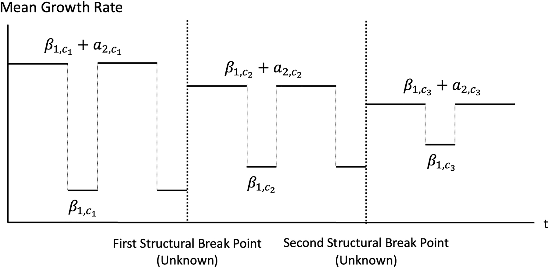
Graphical illustration of the priors for the narrowing gap between mean growth rates during boom and recession.
By substituting equation (36) into equation (35), we obtain
Then, by defining e t = γ 1 + u t and rearranging the terms in equation (39), we obtain:
Empirical Model with Transformed Parameters
where
Lastly, note that structural breaks in the mean growth rates for boom and recession imply structural breaks in the long-run mean growth rate. Based on equation (39), the long-run mean growth rate (τ t ) at each iteration of the MCMC can be obtained by:
where γ 1 can be recovered in the same way as the β 1 coefficient is recovered in footnote 7, with M in footnote 7 now referring to the realized number of mixtures at a particular iteration of the MCMC; I T refers to information up to T; and Pr[S t = 2] refers to the steady-state probability that S t = 2, which is given by Pr[S t = 2] = (1 − p S,11)/(2 − p S,11 − p S,22).
5.2 Empirical Results
Data employed is the seasonally-adjusted postwar U.S. industrial production index, which is obtained from the Federal Reserve Bank of St. Louis economic database (FRED), and the sample covers the period 1947:M1–2019:M9. Figure 3 depicts the growth rate of the industrial production index. We estimate both the proposed model and the model with a normality assumption for the error term. We obtain 500,000 MCMC draws and discard the first 100,000 to guarantee the convergence of the sampler and to avoid the effect of the initial values. All the inferences are based on the remaining 400,000 draws. We first consider the following tight priors:
![Figure 3:
U.S. Industrial production (IP) index growth [1947:M1–2019:M9].](/document/doi/10.1515/snde-2022-0055/asset/graphic/j_snde-2022-0055_fig_003.jpg)
U.S. Industrial production (IP) index growth [1947:M1–2019:M9].
Priors #1: Tight Priors
where the base distribution G
0 specified for the Dirichlet process implies the following unconditional distributions for γ
1 and
which are used as the priors for γ
1 and
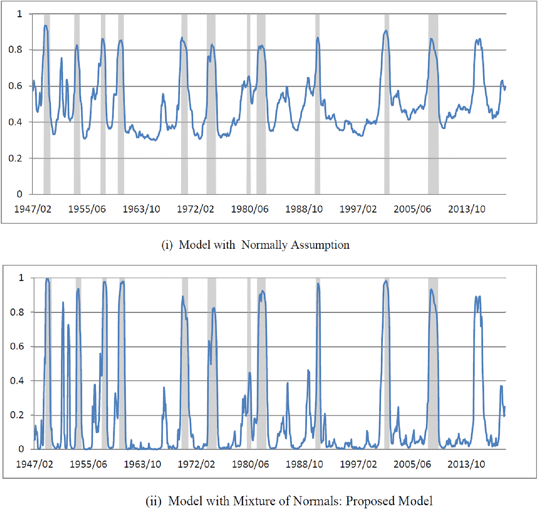
When we apply a normality test to the posterior means of the standardized errors from the model with a normality assumption, the null is rejected at a 5 % significance level. This provides us with a justification for employing the proposed model. For the proposed model, the posterior mean for the number of mixtures turns out to be slightly higher than 3, and the null hypothesis of normality is not rejected (at a 5 % significance level) for the posterior means of the standardized errors.[13] These results suggest that the Dirichlet process mixture normals model reasonably well approximates the unknown distribution of the error term. Furthermore, a Bayesian model selection criterion (Watanabe-Akaike information criterion or WAIC by Watanabe (2010)) very strongly prefers the proposed model to the model with a normality assumption.
Figure 4 depicts the posterior probabilities of recession from the two models under the tight priors. The shaded areas represent the NBER recessions. Estimates of the recession probabilities from the proposed model are much sharper and agree much more closely with the NBER reference cycles than those from a model with a normality assumption.

Posterior probabilities of recession based on the two competing models: Tight priors.
To examine the robustness of the results to the priors employed, we also consider the following loose priors for some of the parameters by keeping the priors for the rest of the parameters unchanged:
Prior #2: Loose Priors
For the case of the loose priors, the prior variances of the parameters are set to be much larger than those for the case of the tight priors. We set the prior means of the parameters to be identical for the two cases. Figure 5 compares the posterior probabilities of recession from the two competing models under the loose priors. For the model with a normality assumption, the inference on the recession probabilities deteriorates considerably with the loose priors. For the proposed model, however, the recession probabilities under the loose priors are almost the same as those under the tight priors, and we continue to have sharp inferences on the recession probabilities. That is, the proposed model is robust to the priors employed, while the model with a normality assumption is very sensitive to the priors.
Posterior probabilities of recession based on the two competing models: Loose priors.
Figure 6 depicts the posterior means of the error volatilities and those of the long-run mean growth rates obtained based on equation (41). These are obtained from the proposed model under the tight priors.[14] As shown in the upper panel of Figure 6, the high and medium volatility regimes are mostly focused on the period before the mid-1980s. In most of the post-1984 period, the low volatility regime dominates except for a few episodes of medium or high volatility that include the Great Recession. The lower panel of Figure 6 demonstrates a pattern for a steadily decreasing long-run mean growth rate, which is consistent with Stock and Watson (2012) and Eo and Kim (2016).
![Figure 6:
Time-varying volatility and long-run mean growth rate of IP: Proposed model [Tight Prior].](/document/doi/10.1515/snde-2022-0055/asset/graphic/j_snde-2022-0055_fig_006.jpg)
Time-varying volatility and long-run mean growth rate of IP: Proposed model [Tight Prior].
Lastly, the upper panel of Figure 7 shows that the posterior distribution of the error term is bimodal before the mixture of normals is controlled for. However, the lower panel of Figure 7 shows that, once the mixture of normals is controlled for, the distribution of the error term is very close to the normal distribution.

Distribution of the standardized errors (solid line: Standardized errors; broken line: Standard Normal).
6 Summary
We provide solutions to the identification problems that are associated with the estimation of a Markov-switching model in which the unknown error distribution is approximated by the Dirichlet process mixture of normals: (i) the problem of label switching for the Markov-switching regime indicator variable; and (ii) the problem of disentangling the Markov-switching regime indicator variable from the serially independent mixture indicator variable. These solutions are very easy to implement in actual applications, and our Monte Carlo experiments show that the proposed identification schemes and MCMC procedure work well.
When the proposed model and the MCMC procedure are applied to the monthly index of industrial production (1947:M1–2019:M9), they provide us with considerably sharper and more accurate inferences on the business cycle turning points than the model with an assumption of the normally distributed error term. In our model, the irregular components that are not related to business conditions are effectively controlled for.
Funding source: University of Washington
Award Identifier / Grant number: Unassigned
Acknowledgment
Kim acknowledges financial support from the Bryan C. Cressey Professorship at the University of Washington.
References
Angelis, L. D., and V. Cinzia. 2017. “A Markov-Switching Regression Model with Nongaussian Innovations: Estimation and Testing.” Studies in Nonlinear Dynamics and Econometrics 21: 1–22. https://doi.org/10.1515/snde-2015-0118.Search in Google Scholar
Bauwens, L., J.-F. Carpantier, and A. Dufays. 2017. “Autoregressive Moving Average Infinite Hidden Markov-Switching Models.” Journal of Business & Economic Statistics 35: 162–82. https://doi.org/10.1080/07350015.2015.1123636.Search in Google Scholar
Bulla, J., S. Mergner, I. Bulla, A. Sesboüé, and C. Chesneau. 2011. “Markov-Switching Asset allocation: Do Profitable Strategies Exist?” Journal of Asset Management 12: 310–21. https://doi.org/10.1057/jam.2010.27.Search in Google Scholar
Chib, S. 1998. “Estimation and Comparison of Multiple Change-Point Models.” Journal of Econometrics 86: 221–41. https://doi.org/10.1016/s0304-4076(97)00115-2.Search in Google Scholar
Clark, T. E. 2009. “Is the Great Moderation over? an Empirical Analysis.” Economic Review: 5–42. Fourth Quarter 2009, Federal Reserve Bank of Kansas City.Search in Google Scholar
Diebold, F. X., J.-H. Lee, and G. C. Weinbach. 1994. “Regime Switching with Time-Varying Transition Probabilities.” In Nonstationary Time Series Analysis and Cointegration, Advanced Texts and Econometrics, edited by C. Hargreaves, 259–305. Oxford and New York: Oxford University Press.10.1093/oso/9780198773917.003.0010Search in Google Scholar
Dueker, M. 1997. “Markov Switching in GARCH Processes and Mean-Reverting Stock-Market Volatility.” Journal of Business & Economic Statistics 15: 26–34. https://doi.org/10.1080/07350015.1997.10524683.Search in Google Scholar
Eo, Y., and C.-J. Kim. 2016. “Markov-Switching Models with Evolving Regime-specific Parameters: Are Booms or Recessions All Alike?” The Review of Economics and Statistics 98: 940–9. https://doi.org/10.1162/rest_a_00561.Search in Google Scholar
Escobar, M., and M. West. 1995. “Bayesian Density Estimation and Inference Using Mixtures.” Journal of the American Statistical Association 90: 577–88. https://doi.org/10.1080/01621459.1995.10476550.Search in Google Scholar
Filardo, A. J. 1994. “Business Cycle Phases and Their Transitional Dynamics.” Journal of Business & Economic Statistics 12: 299–308. https://doi.org/10.1080/07350015.1994.10524545.Search in Google Scholar
Fox, E., E. Sudderth, M. Jordan, and A. Willsky. 2011. “A Sticky HDP-HMM with Application to Speaker Diarization.” Annals of Applied Statistics 5: 1020–56. https://doi.org/10.1214/10-aoas395.Search in Google Scholar
Frühwirth-Schnatter, S. 2001. “Markov Chain Monte Carlo Estimation of Classical and Dynamic Switching and Mixture Models.” Journal of the American Statistical Association 96: 194–209. https://doi.org/10.1198/016214501750333063.Search in Google Scholar
Frühwirth-Schnatter, S. 2006. Finite Mixture and Markov Switching Models. New York: Springer. Springer Series in Statistics.Search in Google Scholar
Gadea-Rivas, M., A. Gomez-Lscos, and G. Perez-Quiros. 2014. The Two Greatest Recession Vs. Great Moderation. Banco de Espana Working Paper No. 1423.10.2139/ssrn.2497536Search in Google Scholar
Hamilton, J. D. 1989. “A New Approach to the Economic Analysis of Nonstationary Time Series and the Business Cycle.” Econometrica 57: 357–84. https://doi.org/10.2307/1912559.Search in Google Scholar
Hamilton, J. D. 2016. “Macroeconomic Regimes and Regime Shifts.” Handbook of Macroeconomics 2: 163–201. https://doi.org/10.1016/bs.hesmac.2016.03.004.Search in Google Scholar
Kaufmann, S. 2015. “K-state Switching Models with Time-Varying Transition Distributions – Does Loan Growth Signal Stronger Effects of Variables on Inflation?” Journal of Econometrics 187: 82–94. https://doi.org/10.1016/j.jeconom.2015.02.001.Search in Google Scholar
Kim, C.-J. 1994. “Dynamic Linear Models with Markov Switching.” Journal of Econometrics 60: 1–22. https://doi.org/10.1016/0304-4076(94)90036-1.Search in Google Scholar
Kim, C.-J., and C. R. Nelson. 1999. “Has the U.S. Economy Become More Stable? A Bayesian Approach Based on a Markov-Switching Model of the Business Cycle.” The Review of Economics and Statistics 81: 608–16. https://doi.org/10.1162/003465399558472.Search in Google Scholar
Neal, R. 2000. “Markov Chain Sampling Methods for Dirichlet Process Mixture Models.” Journal of Computational & Graphical Statistics 9: 249–65. https://doi.org/10.1080/10618600.2000.10474879.Search in Google Scholar
Song, Y. 2014. “Modeling Regime Switching and Structural Breaks with an Infinite Hidden Markov Model.” Journal of Applied Econometrics 29: 825–42. https://doi.org/10.1002/jae.2337.Search in Google Scholar
Stephens, M. 2000. “Dealing with Label Switching in Mixture Models.” Journal of the Royal Statistical Society: Series B 62: 795–809. https://doi.org/10.1111/1467-9868.00265.Search in Google Scholar
Stock, J., and M. Watson. 2012. “Disentangling the Channels of the 2007-09 Recession.” Brookings Papers on Economic Activity 43: 81–156. https://doi.org/10.1353/eca.2012.0005.Search in Google Scholar
Taddy, M., and A. Kottas. 2009. “Markov Switching Dirichlet Process Mixture Regression.” Bayesian Analysis 4: 793–816. https://doi.org/10.1214/09-ba430.Search in Google Scholar
Watanabe, S. 2010. “Asymptotic Equivalence of Bayes Cross Validation and Widely Applicable Information Criterion in Singular Learning Theory.” Journal of Machine Learning Research 11: 3571–94.Search in Google Scholar
West, M., P. Muller, and M. Escobar. 1994. “Hierarchical Priors and Mixture Models with Application in Regression and Density Estimation.” In Aspects of Uncertainty: A Tribute to D. V. Lindley, edited by A. F. M. Smith and P. R. Freeman, 363–86. London: John Wiley and Sons.Search in Google Scholar
© 2023 the author(s), published by De Gruyter, Berlin/Boston
This work is licensed under the Creative Commons Attribution 4.0 International License.
Articles in the same Issue
- Frontmatter
- Editorial
- Editorial Introduction of the Special Issue of Studies in Nonlinear Dynamics and Econometrics in Honor of Herman van Dijk
- Review
- Challenges and Opportunities for Twenty First Century Bayesian Econometricians: A Personal View
- Research Articles
- Markov-Switching Models with Unknown Error Distributions: Identification and Inference Within the Bayesian Framework
- Dynamic Shrinkage Priors for Large Time-Varying Parameter Regressions Using Scalable Markov Chain Monte Carlo Methods
- Matrix autoregressive models: generalization and Bayesian estimation
- Sequential Monte Carlo with model tempering
- Modeling Corporate CDS Spreads Using Markov Switching Regressions
- Combining Large Numbers of Density Predictions with Bayesian Predictive Synthesis
- Bayesian inference for non-anonymous growth incidence curves using Bernstein polynomials: an application to academic wage dynamics
- Bayesian Reconciliation of Return Predictability
- A Dynamic Latent-Space Model for Asset Clustering
- Posterior Manifolds over Prior Parameter Regions: Beyond Pointwise Sensitivity Assessments for Posterior Statistics from MCMC Inference
- Bayesian Flexible Local Projections