Artificial Neural Network-Based Three-dimensional Continuous Response Relationship Construction of 3Cr20Ni10W2 Heat-Resisting Alloy and Its Application in Finite Element Simulation
-
Le Li
 und
Li-yong Wang
und
Li-yong Wang

Abstract
The application of accurate constitutive relationship in finite element simulation would significantly contribute to accurate simulation results, which plays a critical role in process design and optimization. In this investigation, the true stress–strain data of 3Cr20Ni10W2 heat-resisting alloy were obtained from a series of isothermal compression tests conducted in a wide temperature range of 1203–1403 K and strain rate range of 0.01–10 s−1 on a Gleeble 1500 testing machine. Then the constitutive relationship was modeled by an optimally constructed and well-trained back-propagation artificial neural network (BP-ANN). The evaluation of the BP-ANN model revealed that it has admirable performance in characterizing and predicting the flow behaviors of 3Cr20Ni10W2 heat-resisting alloy. Meanwhile, a comparison between improved Arrhenius-type constitutive equation and BP-ANN model shows that the latter has higher accuracy. Consequently, the developed BP-ANN model was used to predict abundant stress–strain data beyond the limited experimental conditions and construct the three-dimensional continuous response relationship for temperature, strain rate, strain, and stress. Finally, the three-dimensional continuous response relationship was applied to the numerical simulation of isothermal compression tests. The results show that such constitutive relationship can significantly promote the accuracy improvement of numerical simulation for hot forming processes.
Introduction
3Cr20Ni10W2 is a typical austenitic heat-resisting alloy extensively applied in marine diesel engine exhaust valves [1, 2] due to its superior corrosion resistance, oxidation resistance, heat resistance and high strength, creep strength. However, exactly because of its high strength and outstanding heat-resistance, it is a hard issue to process 3Cr20Ni10W2 heat-resisting alloy with conventional processing methods. Hence, a special hot working technology electric upsetting is usually employed to fulfill this task [2, 3]. During the electric upsetting process, the flow behaviors of 3Cr20Ni10W2 heat-resisting alloy become extremely complicated due to concomitant hardening and softening behaviors, which mainly include three metallurgical phenomena: dynamic recovery (DRV), dynamic recrystallization (DRX), and work hardening (WH) [4, 5]. The flow behaviors of material are generally represented by constitutive relationship, the intrinsic relationship among the process variables such as stress, strain, strain rate, and temperature. Constitutive relationship is usually applied to the numerical computation to predict the deformation behaviors of material [6]. Accurate constitutive relationship is the premise of reliable numerical computation results. Therefore, how to accurately describe such complex relationship has been a problem arousing more and more attentions.
For decades, numerous researchers have contributed to three types of constitutive models including phenomenological, analytical, and semi-empirical or empirical ones [7]. The analytical constitutive model has the highest computation efficiency and is regarded as the simplest constitutive model. But generally it is difficult to meet all the assumptions, so this model may fail to predict the material flow behaviors correctly. The semi-empirical or empirical constitutive model couples the effect of strain rate and temperature but treats strain in an exclusive way. Usually the effects of strain, strain rate, and temperature are statistically analyzed in a mutually exclusive manner from the data collected in measurements or observations. To obtain accurate prediction results, large amount of experimental data, small regression tolerance and reliable assumptions must be ensured. The phenomenological one is a mathematical model with relatively higher accuracy, but many coefficients in this model need to be calculated based on the experimental data. This model requires many computational and experimental efforts, and its accuracy mainly depends on the regression tolerance and the formula applicability.
Relative to the previous three types of constitutive models, an easier and more adaptable modeling approach, artificial neural network (ANN) has been rapidly developed in recent years and popularly applied in material flow behaviors. ANN, which emulates the structures, mechanisms, and functions of biological neural networks, has a data-driven black-box structure [8] and can automatically learn and grasp the laws of data, even conducted accurate prediction beyond the data already existing. Explicit professional knowledge is not so important for the researchers using ANN model, and the critical work is collecting the data of some typical examples. Most ANNs contain some different “learning rules” to modify the weights of the connections on the basis of the input patterns that it is presented with. The commonly used learning rules mainly include the Hebbian rule, delta rule, competitive learning rule, and anti-Hebbian rule [9], in which the delta rule is often applied in the most widely and successfully used ANN called “back-propagation artificial neural network” (BP-ANN). With BP, “learning” is a supervised process that follows with each cycle through the feed-forward computation of activations and the backward propagation of error signals for weight adjustments via the generalized delta rule [10]. Recently, a lot of efforts have been spent on the hot deformation behaviors and constitutive description of several alloys by BP-ANN model. Liu J et al. [11], Phaniraj M P et al. [12], Mandal S et al. [13], Lin Y C [14] et al. conducted BP-ANN models to predict the flow behaviors of high-speed steel, carbon steels, type 304 L stainless steel, 42CrMo steel, etc. These reports about BP-ANN revealed that BP-ANN is an effective tool to predict the complex non-linear hot flow behaviors by self-training to be adaptable to the material characteristics.
As for 3Cr20Ni10W2 heat-resisting alloy, there are few reports of the constitutive modeling of the hot flow behaviors by BP-ANN. As is known, the stress–strain data amount and accuracy input into the finite element (FE) model have a significant influence on the simulation accuracy of the hot forming processes. The BP-ANN meets this request just right since it has not only high characterization accuracy but also high predictability. In this work, the stress–strain data for 3Cr20Ni10W2 heat-resisting alloy in wide deformation conditions were predicted by BP-ANN to construct the constitutive relationship with a new style: 3D continuous response relationship. Such constitutive relationship reflects the 3D continuous response of stress to strain, strain rate, and temperature in extensive deformation and was exhibited as a 3D continuous interaction space. The 3D continuous interaction space is digital, which means the stress values under any temperatures, strain rates, and strains can be read and accessed as long as the corresponding deformation conditions are within the scope of this space. The accuracy of such 3D continuous response relationship is strongly guaranteed by the high accuracy of BP-ANN model.
This work focused on the 3D continuous response relationship construction of 3Cr20Ni10W2 heat-resisting alloy using BP-ANN model and its application in accuracy improvement of FE numerical simulation. The core of the FE model with high accuracy is the accurate constitutive relationship in wide ranges of temperature, strain, and strain rate. In this research, this is guaranteed by a well-trained BP-ANN model taking temperature (T), strain rate (
Experimental procedures
The detailed chemical compositions of 3Cr20Ni10W2 heat-resisting alloy are as follows (wt. %): Cr 20, Ni 10, W 2, Si 1, C 0.25, and balance Fe. From the raw material, totally 20 cylinders with diameter of 10 mm and height of 12 mm were machined as the specimens by wire-electrode cutting. The experimental procedures of isothermal compression tests formulated according to ASTM Standard: E209-00 were shown in Figure 1. According to the schedule, these specimens were firstly heated to 1373 K and held for 12 h in a furnace to obtained homogenized microstructures. In order to accurately control the temperature in the test, two K-type thermocouple wires were welded on the specimen before the test to record the real-time temperature of the specimen. Then the specimens were respectively fixed at the exact center of the anvils on a computer-controlled, servo-hydraulic Gleeble 1500 testing machine, heated to designated temperatures (1203 K, 1253 K, 1303 K, 1353 K and 1403 K) with a fixed heating rate of 5 K/s and kept in these temperatures for 180 s to reduce anisotropy and eliminate internal temperature gradients. Subsequently, these specimens were respectively compressed to 40 % height with the strain rates of 0.01 s−1, 0.1 s−1, 1 s−1 and 10 s−1. After the isothermal compression tests, the specimens were water quenched immediately to keep the deformed microstructures at elevated temperature. In the tests, a computer control automatic data acquisition system was used to monitor the experimental data continuously. The recorded normal stress and normal strain were converted into homologous true stress and true strain according to the formulae:
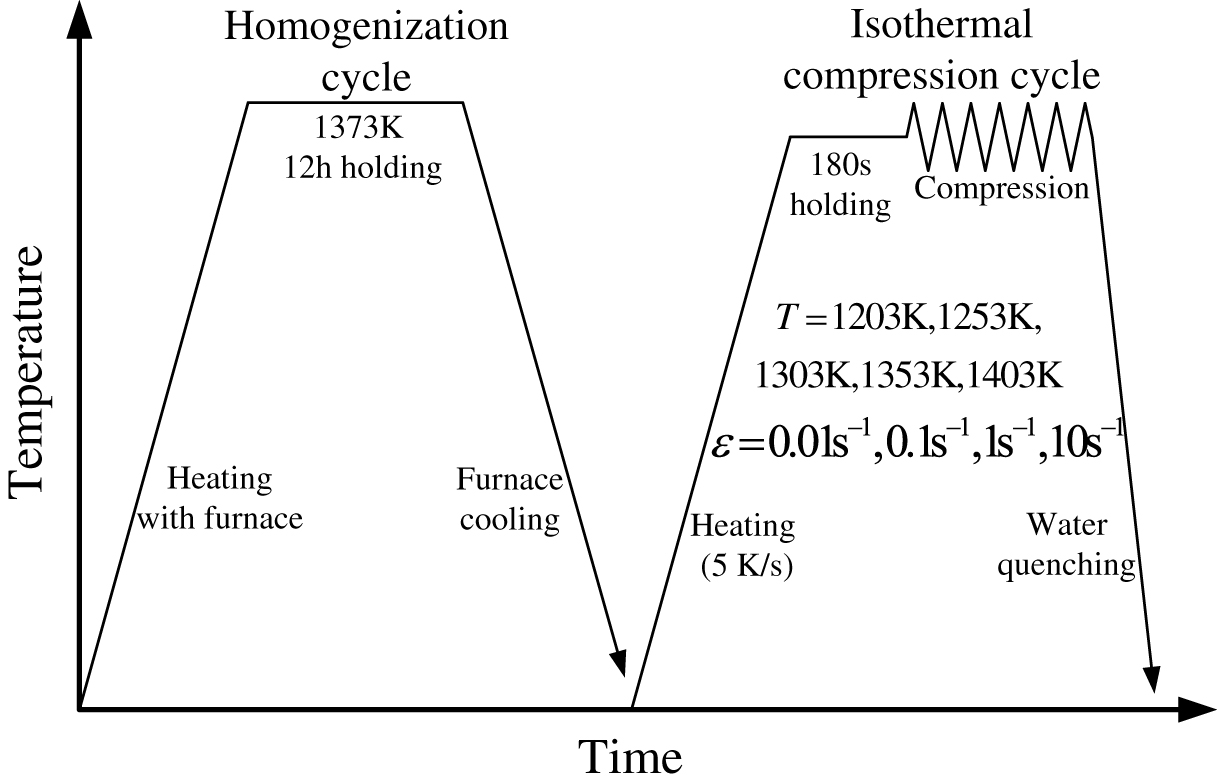
Experimental procedures for the isothermal compression tests.
Flow behaviors characteristics
The true stress–strain data of 3Cr20Ni10W2 heat-resisting alloy measured by previous isothermal compression tests were shown in Figure 2. As expected, stress–strain relationship is highly non-linear, and highly susceptible to three parameters including temperature, strain, and strain rate. By comparison of one stress–strain curve with another, it can be summarized that the stress level decreases with temperature increases or strain rate decreases. This is due to the following facts. When the strain rate is accelerated, the dislocations participating in deformation in unit time increase, in this situation, deformation is unable to be coordinated duly by dislocation and grain movements, thus, the multiplication of dislocation push the stress value to a higher level. The multiplication of dislocation leads to the improvement of stress level. When raising the deformation temperature level, the heat activation increases the average kinetic energy in atoms and makes the atomic diffusion and dislocation movement easier. And this induces the decrease of stress level. As for each stress–strain curve, it shows an initial rapid and the following more and more slow work hardening (WH), following which two types of stress–strain evolution exist. In the first case, the stress decreases gradually after a single peak value, an evidence of dynamic recrystallization (DRX) softening, which corresponds to the conditions of 0.01 s−1 & 1203–1253 K, 0.1 s−1 & 1203–1303 K, 1 s−1 & 1203–1353 K and 10 s−1 & 1203–1403 K. In the second case, the stress approximately keeps a steady state, an evidence of dynamic recovery (DRV) softening, under the conditions of 0.01 s−1 & 1303–1403 K, 0.1 s−1 & 1353–1403 K and 1 s−1 & 1403 K. From the previous descriptions, it can be concluded that the compression flow behaviors of 3Cr20Ni10W2 alloy are extremely complex and highly non-linear, not only due to the effects of temperature and strain rate to stress level, but also due to the evolution characteristics involving WH, DRX, and DRV indicated in each stress–strain curve.

The stress–strain curves of 3Cr20Ni10W2 heat-resisting alloy under different temperatures with the strain rates of (a) 0.01 s−1, (b) 0.1 s−1, (c) 1 s−1 and (d) 10 s−1.
Establishment and evaluation of BP-ANN model
Development of BP-ANN model
Because of the complexity described above, it is a difficult issue to characterize the flow behaviors accurately. A BP-ANN model for the isothermal compression flow behaviors of 3Cr20Ni10W2 heat-resisting alloy in respect of dependency of strain, strain rate, and temperature, was developed by taking deformation temperature (T), strain rate (
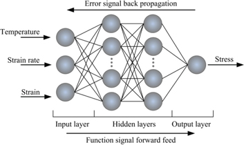
The schematic representation of the BP-ANN architecture.
It is common that the determination of the appropriate number of hidden layers and neurons in each hidden layer is one of the most critical tasks in obtaining an accurate BP-ANN model. It was assumed that the network structure with one or two hidden layers was adopted to test respectively, and then the appropriate number needed to be finally determined through the appropriate tolerance evaluation between the predicted and experimental data. An indicator of mean square error (MSE) as eq. (1) [16] was introduced to evaluate the training performance and the generalization performance of the BP-ANN, and accordingly the optimal hidden layer number and neuron number would be determined by comparing the performance of different networks deriving from different network structure parameters. It is noted that smaller MSE-value indicates better network performance. As for two different network structures, i. e. one or two hidden layers, the relative MSE plots along with the number of neurons in each hidden layer were calculated respectively as shown in Figure 4. The comparison of the MSE plots between the different network structures in Figure 4 shows that the structure of two hidden layers induces lower MSE-value level, and thus it possesses higher generalization performance. Focusing on the cases with two hidden layers, the MSE-value declines with neuron number increasing, while it appears an inverse trend when the neuron number is above 9, which indicates that increasing neuron number up till 9 elevates the network performance significantly. Above all, two hidden layers and 9 neurons in each hidden layer are determined for the final network architecture.
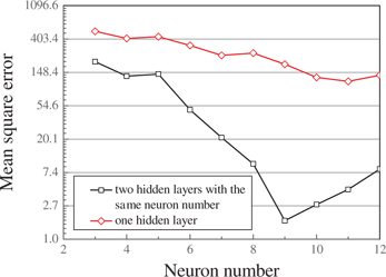
The influences of the hidden layer number and neuron number in each hidden layer on the generalization performance of the neural network.
where Ei is an experimental stress value; Pi is a predicted stress value; N is the number of data samples.
It is noteworthy that the numerical values of the input and output variables distribute in distinct ranges and even dimensions, which induces the poor convergence speed and prediction accuracy of a BP-ANN model. Hence, a normalization process for initial true stress–strain data is essential to ensure the input and output variables being dimensionless and being in an approximately same magnitude. In this research, the normalization processing was realized by eq. (2). The coefficients of 0.05 and 0.25 in eq. (2) are regulating parameters for the sake of narrowing the magnitude of the normalized data within 0 to 0.3. It had been demonstrated by a trial and error method that such a magnitude could bring the promotions in convergence speed and prediction accuracy. Besides, ahead of the normalization processing, the logarithm style was adopted for the initial strain rates, which exhibit large magnitude distinction and may induce considerable errors.
in which x is the experimental value of input or output variable; xmin and xmax are respectively the minimum and the maximum values of input and output variable; xn is the normalization value.
In the present network, transfer functions of the hidden layers and the output layer were empirically chosen as tansig function and purelin function. The training function and the learning function adopted Trainbr function and learngd function respectively.
It is well accepted that learning rate directly determines the revised value of weight in each training cycle, simultaneously plays an important role in the convergence property of networks. Commonly, a high learning rate may cause instability in training, while conversely may get low convergence speed but could keep off the local least values and approach the true least error. Consequently, a lower learning rate is usually selected for better stability and convergence property, and 0.02 was applied in the present network. In addition, the goal of training error before anti-normalization processing was set as 0.0001.
Evaluation of BP-ANN model
To synthetically estimate the prediction capability of BP-ANN model, two commonly used statistical indicators of correlation coefficient (R) and average absolute relative error (AARE) [17], which were expressed as eqs (3) and (4), were introduced. A high R-value close to 1 illustrates that the predicted values conform to the experimental ones well, meanwhile, a low AARE-value close to 0 indicates that the sum of the errors between the predicted and experimental values tends to be 0. Thereby, such R and AARE are expected.
in which E and P are respectively experimental value and predicted value of true stress;
Using the well-trained BP-ANN model, the true stress values under experimental conditions which include the deformation conditions corresponding to the previous training points and test points were predicted. After that, the correlation relationships between the experimental and predicted true stress were expressed in Figure 5. Each point in Figure 5 takes experimental stress and predicted stress as horizontal and vertical axis respectively. The straight line at 45 degrees from the axes is the best linear fit line. If the experimental stress is equal to predicted stress, the corresponding point would lie on this line. It is clearly observed that the points in Figure 5, especially the ones in Figure 5(a), lie very close to the ideal line, indicating well consistency between the experimental and predicted results. In addition, the R-values for the training part and test part are respectively 0.9992 and 0.9981. As stated above, such high values of correlation coefficient R suggest that the predicted stress values conform very well to the experimental ones in an alternative way. Besides, the AAREs were calculated as well. The AARE-value deriving from the test part is 1.7948 %, while that for the training part is merely 0.3314 %. Such minor errors bode the high accuracy exhibited in the training and test work by BP-ANN.
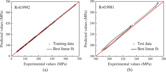
The correlation relationships between the predicted and experimental true stress for the (a) training part and (b) test part.
The relative error (δ) [13] in eq. (5) represents the percentage error of each predicted stress–strain value relative to the homologous experimental value, in order to further and more detailedly evaluate the BP-ANN model, it was introduced. In the training part, the relative errors range from −2.92 % to 2.80 %, and for the test part their distribution range is from −0.51 % to 2.10 %. Figure 6 expresses the columnar distribution maps of the relative errors in the training and test part. In terms of Figure 6, it is not so difficult to find that the relative errors, no matter in training or test part, are within a narrow range of 0±3 %. However, it is more noteworthy that the most of the δ-values are miraculously concentrated in the vicinity of the ideal value 0: in the training part, the δ-values of 92.8 % points are within the interval of [−1 %, 1 %], and for the test part, 48.2 % are concentrated in [−1 %, 1 %], at the same time, 94.5 % are concentrated in [−1 %, 2 %]. These results arisen from unbiased statistical data provide direct evidence that high precision both in the training and test stage was acquired by the BP-ANN model.
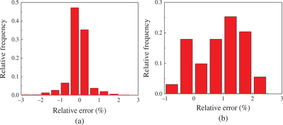
The relative error distributions of the predicted true stress corresponding to (a) the training points and (b) the test points.
where Pi is a predicted stress value and Ei is homologous experimental stress value.
Figure 7 shows the stress–strain data predicted by the BP-ANN model and their comparisons with the initial experimental curves. Obviously, the predicted data can grasp the stress–strain evolution rules precisely, that is, the stress decreases with temperature increasing or strain rate decreasing, predictably indicating that the present BP-ANN model is able to track the work hardening and dynamic softening regions of 3Cr20Ni10W2 heat-resisting alloy. Moreover, as shown in Figure 7, the predicted points on the eighteen training curves almost coincide with the experimental stress–strain curves. Compared with the predicted points on the training curves, the predicted points on the test curves of 1253 K & 0.1 s−1 and 1303 K & 1 s−1 have relatively larger deviations. Nevertheless, the maximum relative error is merely 2.10 %, a quite acceptable value. By comparing the predicted and experimental true stress corresponding to training points and test points, the learning and generalization capabilities of BP-ANN model were validated respectively. Conclusively, the present BP-ANN model has admirable performance in describing and predicting the true stress of 3Cr20Ni10W2 heat-resisting alloy.
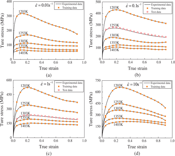
The comparison between the experimental and predicted true stress by the BP-ANN model at different temperatures and the strain rate of (a) 0.01 s−1, (b) 0.1 s−1, (c) 1 s−1 and (d) 10 s−1.
Introduction of the improved Arrhenius-type constitutive equation
Over the past decades, the Arrhenius-type constitutive equation, a type of phenomenological constitutive model, was widely used to describe the constitutive relationship completely omitting the effect of strain. While, the strain is a vital parameter in hot forming processes and has a critical influence on the flow behaviors, especially for those strain sensing materials. Therefore, the previous Arrhenius-type constitutive equations often received poor results, until a revised model taking the influence of strain into account was put forward and successfully utilized to accurately describe the deformation behaviors of 42CrMo steel under high temperature by Lin Y C et al. [16]. Subsequently, this kind of improved Arrhenius-type constitutive equation was successfully applied in constitutive relationship descriptions of various materials [18, 19, 20] due to such superiority.
In Ref [21], Quan et al. calculated and reported the improved Arrhenius-type constitutive equation of 3Cr20Ni10W2 heat-resisting alloy, and it was expressed in eq. (6).
where
The polynomial fit results of
| B0 | 1412.935 | C0 | 14.297 | D0 | 130.349 | E0 | 5.266 |
| B1 | −15062.484 | C1 | −192.193 | D1 | −1432.610 | E1 | −9.324 |
| B2 | 132589.938 | C2 | 1673.660 | D2 | 12583.389 | E2 | 52.670 |
| B3 | −647327.386 | C3 | −8064.572 | D3 | −61273.071 | E3 | −182.396 |
| B4 | 1.864E6 | C4 | 23120.881 | D4 | 176160.403 | E4 | 504.786 |
| B5 | −3.258E6 | C5 | −40386.571 | D5 | −307513.349 | E5 | −977.292 |
| B6 | 3.396E6 | C6 | 42156.082 | D6 | 320366.422 | E6 | 1166.278 |
| B7 | −1.942E6 | C7 | −24152.987 | D7 | −183116.203 | E7 | −762.116 |
| B8 | 468636.323 | C8 | 5841.327 | D8 | 44185.280 | E8 | 210.366 |
Prediction capability comparison between the BP-ANN model and Arrhenius-type constitutive equation
The experimental stress–strain curves and stress–strain points predicted by the Arrhenius equation were plotted in Figure 8. It is easy to find that the stress–strain points predicted by the constitutive equation are in qualitative agreement with the stress–strain evolution rules. But relative to the experimental stress–strain curves, these predicted points appear notable deviations, especially under the temperature of 1203 K and 1253 K. Moreover, such deviations are significantly larger than the predicted stress–strain data by BP-ANN model in Figure 7. For the sake of more intuitive contrast of prediction accuracy between these two models, the AARE-values and R-values relative to the experimental true stress were calculated by eqs (3) and (4). According to the calculation results, it is manifest that the AARE-value and R-value for the BP-ANN model are 0.401 % and 0.9989, but for the constitutive equation, they are 4.08 % and 0.995. Lower AARE-value and higher R-value indicate that the BP-ANN model has higher accuracy in predicting the true stress of 3Cr20Ni10W2 heat-resisting alloy than the constitutive equation. It is noteworthy that the experimental data on the test curves corresponding to 1253 K & 0.1 s−1 and 1303 K & 1 s−1, which participated in the construction of constitutive equation, are exactly not involved in the training data of the BP-ANN model. Even so, the BP-ANN model still exhibits dramatic predominance, further proving its superiority in constitutive relationship description and prediction. Quan et al. have obtained similar conclusions when constructing the constitutive relationships of AZ80 magnesium alloy [22]. The reason why the constitutive equation cannot follow the tracks of varied true stress so effectively as the BP-ANN model is that the constitutive equation needs to take the physical interpretation into account. Yet, on the contrary, the BP-ANN model can just predict the true stress under different deformation conditions regardless of the physical interpretation, and the essential tasks are preparing proper training and test data, afterward developing the optimal network structure and parameters for the BP-ANN model.
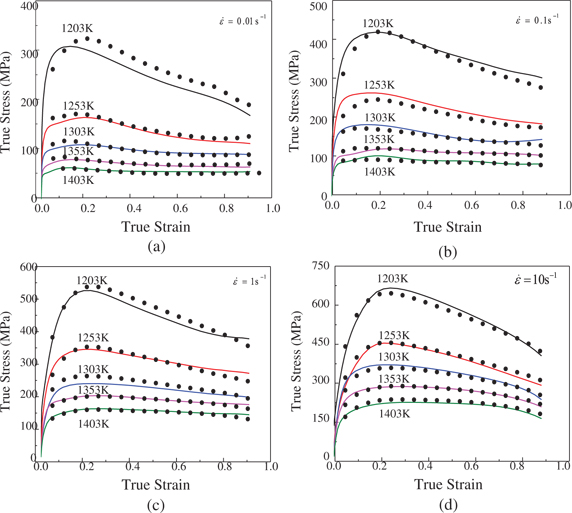
The comparisons between the experimental (curves) and predicted (black circles) true stress by the Arrhenius-type constitutive equation under the strain rates of (a) 0.01 s−1, (b) 0.1 s−1, (c) 1 s−1 and (d) 10 s−1.
Construction of 3D continuous response relationship
As stated above, the BP-ANN model is highly reliable and more accurate than the improved Arrhenius-type constitutive equation. Therefore, due to outstanding generalization capability of the BP-ANN model, it can undoubtedly be employed to predict the true stress of 3Cr20Ni10W2 heat-resisting alloy outside of the experimental conditions. In this investigation, the true stress–strain data under the temperature range of 1103–1403 K, the strain rate range of 0.01–10 s−1, as well as the strain range of 0.05–0.9 were predicted. The predicted results were expressed as three-dimensional continuous response relationship among strain, strain rate, temperature and stress (illustrated in Figure 9). In Figure 9, the X-axis, Y-axis, Z-axis and V-axis respectively represent deformation temperature, strain rate, true strain and true stress. The values on V-axis, that is, the predicted true stress values under different deformation conditions are indicated by different colors. Figure 9(a) is a 3D continuous interaction space, a global expression of the 3D continuous response relationship. It covers all the deformation conditions and homologous predicted true stress values. Therefore, any true stress values in the deformation condition scope of 3D continuous interaction space can be read and accessed directly. It is also possible to implant the ANN model into the finite element software by program codes, such as Msc.Marc [23]. Thus, the software can directly extract the required stress values and input them into computation system. Figure 9(b)–(d), which were constructed by cutting the 3D continuous interaction space into slices along with the X-axis, Y-axis, Z-axis, respectively intensively reflect the 3D continuous response relationships under the fixed temperatures, strain rates and strains.
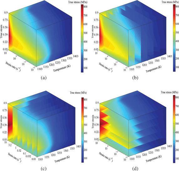
The 3D relationship among temperature, strain rate, strain and stress: (a) 3D continuous interaction space; 3D continuous response relationship under fixed (b) temperatures, (c) strain rates and (d) strains.
It is well known that the stress–strain data play an critical role in many studies, such as the DRX kinetics model [24], processing maps [25], ductile fracture criteria [26], etc. In these studies, the amount and quality of stress–strain data have a significant influence on the research results. Exactly, the 3D continuous response relationship constructed in this paper can provide abundant and accurate stress–strain data in extensive scope for the relevant studies on 3Cr20Ni10W2 heat-resisting alloy to guarantee the creditability of research findings. Beyond that, the 3D continuous response relationship plays an essential part in finite element method (FEM). As is known, the stress–strain data are the most fundamental data to predict the deformation behaviors of materials with FEM. On the basis of the 3D continuous response relationship, it is realizable to perform accurate numerical simulations of various hot forming processes. In this way, more reasonable design and optimization of the process parameters such as the deforming temperature, the shape of die cavity, deformation velocity, etc., can be conducted.
Application in FEM of BP-ANN model
During hot deformation processes, the materials would experience extensive temperature and strain rate regions. Thus, the accurate numerical simulation of hot forming processes naturally needs a great deal of stress–train data in wide deformation conditions. However, the measurement of experimental data is undoubtedly a time-consuming and effort-consuming task. In such situation, the accurate prediction of stress–strain data outside of experimental conditions can actually help a lot. In this investigation, the response relationship among forming parameters predicted by the well-trained BP-ANN model were implanted in the finite element solver to simulate the isothermal compression tests of 3Cr20Ni10W2 heat-resisting alloy under the deformation conditions of 1203 K & 0.01, 0.1, 1 and 10 s−1. The established FE model was presented in Figure 10. In the FE model, the anvils and specimen were respectively defined as rigid objects and plastic object. During the actual isothermal compression process in Gleeble 1500 test machine, constant temperature is qualitatively ensured for the specimen, so the heat transfer and thermal radiation of the specimen with the anvils and environment as well as the work-heat conversion were ignored in the present FE model. Besides, a constant shear friction coefficient of 0.1 was set to conform to the practical graphite lubricant on the contact surfaces between the anvils and specimen. To meet the demand of fixed strain rates, the compression velocity of the driver anvil (anvil I) was defined according to eq. (8) [27]. The compression rate was 60 %, which corresponds to 7.2 mm height reduction of the specimen.
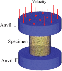
The finite element model for the simulated isothermal compression tests of 3Cr20Ni10W2 heat-resisting alloy.
where v stands for the instantaneous compression velocity of the driver anvil; h0 is the original height of the specimen, and here h0=12 mm;
The effective strain and effective strain rate distributions of the specimens sectioned along the axial direction were presented in Figures 11 and 12. From Figure 11, it can be seen that the deformation of the specimen is inhomogeneous due to the friction between the specimen and anvils. The specimen can be broadly divided into hard deformation region, small deformation region and severe deformation region. The friction between the specimen and anvils and constraint of anvils would significantly reduce the material flowabilities of the vicinity region of the end plane, so this region is hard deformation region. The central region is slightly affected by the friction, and the extrusion of the hard deformation region would greatly promote the material flow of this region, thus, large deformation would occur in the central region and it is defined as severe deformation region. As for the vicinity region of the cylindrical surface, it is almost not affected by the friction and the extrusion of other regions. The material in this region is roughly in a state of uniaxial compression, and the deformation degree is between the ones of hard deformation region and severe deformation region, so the vicinity region of the cylindrical surface is small deformation region. These simulation results are in well agreement with the real deformation circumstances of the isothermal compression tests. Besides, the effective strain of the severe deformation regions under the temperature of 1203K and strain rate of 0.01, 0.1, 1 and 10 s−1 are all about 0.92, and the effective strain rates also reach the corresponding values of 0.01, 0.1, 1 and 10 s−1 respectively, which indicate that the simulated process parameters can actually reflect the real experimental conditions.
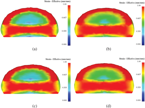
The effective strain distributions under the temperature of 1203 K and strain rate of (a) 0.01 s−1, (b) 0.1 s−1, (c) 1 s−1 and (d) 10 s−1.
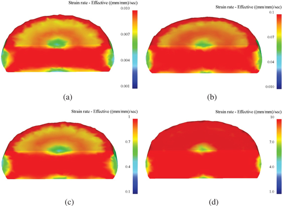
The effective strain rate distributions under the temperature of 1203 K and strain rate of (a) 0.01 s−1, (b) 0.1 s−1, (c) 1 s−1 and (d) 10 s−1.
Corresponding to the above simulation experiments with the predicted stress–strain response relationship by BP-ANN model, the controlled simulation experiments using the stress–strain data measured from isothermal compression tests were also conducted. Subsequently, the stroke-load curves data were exported from the FE solver. And the continuously monitored stroke-load curves by the automatic data acquisition system in the compression tests are assumed to be the ideal curves. The comparisons between the simulated stroke-load curves using different stress–strain data and the ideal curves were presented in Figure 13. From Figure 13, it is known that the simulated evolution rules of forming load with stroke are approximately in accordance with the experimental ones, indicating that the numerical simulation can indeed provide some guidance and reference for the practical processes. However, it is obvious that the predicted stroke-load curves with the predicted stress–strain response relationship by BP-ANN model lie more close to the experimental curves from the global aspect. Especially when the stroke is above 3 mm, the simulated stroke-load curves with the experimental stress–strain data more and more diverge from the ideal curves, but the ones with predicted stress–strain response relationship by BP-ANN model can track the ideal curves in relatively high accuracy all along. It is valuable to note that, when the stroke is below 1 mm, all the simulation results appear relatively larger deviations from the ideal ones. This lies in the fact that the elastic deformation stage corresponding to the true strain below 0.05 was ignored in the stress–strain data or response relationship imported in FE solver. Nevertheless, such small errors can be negligible in the most of hot forming processes with large deformation such as extrusion, forging and rolling. The above comparison gives the full proof that the present response relationship constructed by the BP-ANN model can significantly improve the numerical simulation accuracy of hot forming processes.
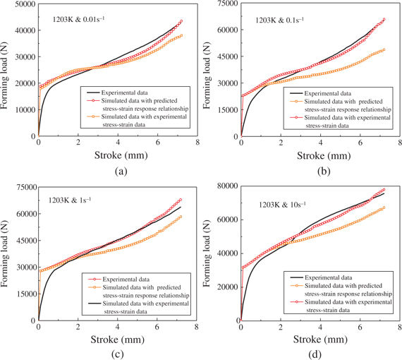
Comparisons between the predicted and experimental stroke-load curves under the temperature of 1203 K and strain rates of (a) 0.01 s−1, (b) 0.1 s−1, (c) 1 s−1 and (d) 10 s−1.
Conclusions
The true stress level of 3Cr20Ni10W2 heat-resisting alloy decreases with increasing temperature or decreasing strain rate. The true stress varies along with strain highly non-linearly, which represents the non-linear variation of the comprehensive effects of different action mechanisms including dynamic recrystallization, dynamic recovery and work hardening.
A BP-ANN model taking the deformation temperature (T), strain rate (
The three-dimensional continuous response relationship within the temperature range of 1103–1403 K, the strain rate range of 0.01–10 s−1, and the strain range of 0.05–0.9 was predicted. Such constitutive relationship can provide abundant and accurate stress–strain data in extensive scope for the FE model of 3Cr20Ni10W2 heat-resisting alloy.
The simulated isothermal compression tests under the temperature of 1203 K and strain rates of 0.01 s−1, 0.1 s−1, 1 s−1 and 10 s−1 were conducted in the FE solver. The comparison between the simulated stroke-load curves based on the experimental stress–strain data and predicted stress–strain response relationship revealed the fact that the constitutive relationship constructed by the BP-ANN model can significantly improve the numerical simulation accuracy of hot forming processes.
Funding statement: This work was supported by the project of National Natural Science Foundation of China (No.51605035), Beijing finance found of science and technology planning project (KZ201611232032) (KM20161123200), and young prominent talent projects. (2014000026833ZK25).
References
[1] G.Z. Quan, J.T. Liang, Y.Y. Liu, G.C. Luo and J. Zhou, Mater. Des., 52 (2013) 593–601.10.1016/j.matdes.2013.05.085Suche in Google Scholar
[2] T. Moriyama, Y. Izaki, K. Umeda, R. Oka, Y. Nishioka and T. Tanaka, Mater. Sci. Tech-Lond., 10 (1994) 993–1001.10.1179/mst.1994.10.11.993Suche in Google Scholar
[3] N. Biba, A. Lishnij and A. Vlasov, J. Mater. Process. Technol., 80 (1998) 184–187.10.1016/S0924-0136(98)00139-3Suche in Google Scholar
[4] Y.C. Lin and X.-M. Chen, Mater. Des., 32 (2011) 1733–1759.10.1016/j.matdes.2010.11.048Suche in Google Scholar
[5] Y.C. Lin, M.S. Chen and J. Zhong, Comp. Mater. Sci., 43 (2008) 1117–1122.10.1016/j.commatsci.2008.03.010Suche in Google Scholar
[6] G.Z. Quan, J. Pan and X. Wang, Appl. Sci., 6 (2016) 66.10.3390/app6030066Suche in Google Scholar
[7] D. Samantaray, S. Mandal, A.K. Bhaduri, S. Venugopal and P.V. Sivaprasad, Mater. Sci. Eng. A, 528 (2011) 1937–1943.10.1016/j.msea.2010.11.011Suche in Google Scholar
[8] G.-Z. Quan, W.-Q. Lv, Y.-P. Mao, Y.-W. Zhang and J. Zhou, Mater. Des., 50 (2013) 51–61.10.1016/j.matdes.2013.02.033Suche in Google Scholar
[9] X. Yao, Proc. IEEE, 87 (1999) 1423–1447.10.1109/5.784219Suche in Google Scholar
[10] S. Singh, V. Vashishtha and T. Singla, Int. J. Res., 1 (2014) 934–942.Suche in Google Scholar
[11] J. Liu, H. Chang, T.Y. Hsu and X. Ruan, J. Mater. Process. Technol., 103 (2000) 200–205.10.1016/S0924-0136(99)00444-6Suche in Google Scholar
[12] M.P. Phaniraj and A.K. Lahiri, J. Mater. Process. Technol., 141 (2003) 219–227.10.1016/S0924-0136(02)01123-8Suche in Google Scholar
[13] S. Mandal, P.V. Sivaprasad, S. Venugopal and K.P.N. Murthy, Appl. Soft Comput., 9 (2009) 237–244.10.1016/j.asoc.2008.03.016Suche in Google Scholar
[14] Y.C. Lin, J. Zhang and J. Zhong, Comp. Mater. Sci., 43 (2008) 752–758.10.1016/j.commatsci.2008.01.039Suche in Google Scholar
[15] Y. Zhu, W. Zeng, Y. Sun, F. Feng and Y. Zhou, Comp. Mater. Sci., 50 (2011) 1785–1790.10.1016/j.commatsci.2011.01.015Suche in Google Scholar
[16] Y.C. Lin, M.S. Chen and J. Zhang, Mater. Sci. Eng. A, 499 (2009) 88–92.10.1016/j.msea.2007.11.119Suche in Google Scholar
[17] S. Mandal, V. Rakesh, P.V. Sivaprasad, S. Venugopal and K.V. Kasiviswanathan, Mater. Sci. Eng. A, 500 (2009) 114–121.10.1016/j.msea.2008.09.019Suche in Google Scholar
[18] Z.J. Pu, K.H. Wu, J. Shi and D. Zou, Mater. Sci. Eng. A, 192 (1995) 780–787.10.1016/0921-5093(94)03314-5Suche in Google Scholar
[19] F.A. Slooff, J. Zhou, J. Duszczyk and L. Katgerman, Scripta Mater., 57 (2007) 759–762.10.1016/j.scriptamat.2007.06.023Suche in Google Scholar
[20] N. Haghdadi, A. Zarei-Hanzaki and H.R. Abedi, Mater. Sci. Eng. A, 535 (2012) 252–257.10.1016/j.msea.2011.12.076Suche in Google Scholar
[21] G.Z. Quan, Y.P. Mao, C.T. Yu, W.Q. Lv and J. Zhou, Mater. Res., 17 (2014) 451–460.10.1590/S1516-14392014005000016Suche in Google Scholar
[22] G.Z. Quan, Z.H. Zhang, J. Pan and Y.F. Xia, Mater. Res., 18 (2015) 1331–1345.10.1590/1516-1439.040015Suche in Google Scholar
[23] G.Z. Quan, S.A. Pu, Z.Y. Zhan, Z.Y. Zou, Y.Y. Liu and Y.F. Xia, Int. J. Precis. Eng. Man., 16 (2015) 2129–2137.10.1007/s12541-015-0275-ySuche in Google Scholar
[24] A. Dehghan-Manshadi, M.R. Barnett and P.D. Hodgson, Mater. Sci. Eng. A, 485 (2008) 664–672.10.1016/j.msea.2007.08.026Suche in Google Scholar
[25] P. Zhang, C. Hu, C.-G. Ding, Q. Zhu and H.-Y. Qin, Mater. Des., 65 (2015) 575–584.10.1016/j.matdes.2014.09.062Suche in Google Scholar
[26] S.V.S.N. Murty, B.N. Rao and B.P. Kashyap, J. Mater. Process. Technol., 147 (2004) 94–101.10.1016/j.jmatprotec.2003.12.002Suche in Google Scholar
[27] G.Z. Quan, J. Pan and Z.H. Zhang, Mater. Des., 94 (2016) 523–535.10.1016/j.matdes.2016.01.068Suche in Google Scholar
© 2018 Walter de Gruyter GmbH, Berlin/Boston
This article is distributed under the terms of the Creative Commons Attribution Non-Commercial License, which permits unrestricted non-commercial use, distribution, and reproduction in any medium, provided the original work is properly cited.
Artikel in diesem Heft
- Frontmatter
- Research Article
- Effect of Trailing Intensive Cooling on Residual Stress and Welding Distortion of Friction Stir Welded 2060 Al-Li Alloy
- Short Communication
- Study on the Growth Mechanism of K2Ti4O9 Crystal
- Research Articles
- Artificial Neural Network-Based Three-dimensional Continuous Response Relationship Construction of 3Cr20Ni10W2 Heat-Resisting Alloy and Its Application in Finite Element Simulation
- Influence of Thermal Ageing on Microstructure and Tensile Properties of P92 Steel
- A Novel Process for Joining Ti Alloy and Al Alloy using Two-Stage Sintering Powder Metallurgy
- Modeling and Finite Element Analysis for the Dynamic Recrystallization Behavior of Ti-5Al-5Mo-5V-3Cr-1Zr Near β Titanium Alloy During Hot Deformation
- Study on Dynamic Development of Three-dimensional Weld Pool Surface in Stationary GTAW
- Influence of Heat Treatment on Fracture Toughness and Wear Resistance of Nicral-Zro2 Multilayered Thermal Barrier Coating
- Kinetic Study on Phosphate Enrichment Behavior in CaO–SiO2–FeO–Fe2O3–P2O5 Steelmaking Slags
- Effect of Prestrain on Precipitation Behaviors of Ti-2.5Cu Alloy
- Study on Gamma Prime and Carbides of Alloy A286 by Traditional Thermodynamic Calculation