Definition, identification, and estimation of the direct and indirect number needed to treat
-
Valentin Vancak
 und
Arvid Sjölander
und
Arvid Sjölander

Abstract
Objectives
The number needed to treat (NNT) is a widely used efficacy and effect-size measure in epidemiology and meta-analysis, originally defined as the average number of patients who need be treated to obtain one additional beneficial outcome. In this study, we introduce novel direct and indirect formulations of the NNT, the number needed to be exposed (NNE) and the exposure impact number (EIN) - quantifying the average number needed to treat (expose) to achieve benefit via the treatment's direct and indirect effects in the respective treatment group.
Methods
Using nested potential outcomes, we formally define the direct effect NNT, NNE, and EIN (DNNT, DNNE, and DEIN, respectively) and the indirect effect NNT, NNE, and EIN (INNT, INNE, and IEIN, respectively). We then derive their identification conditions in observational studies. We introduce an estimation method and illustrate it with two analytical examples.
Results
The identification results provide explicit conditions under which the novel direct and indirect indices are estimable in observational studies. Simulation studies demonstrate that the proposed estimators are consistent and that the associated analytic confidence intervals attain their nominal coverage rates. Two analytical examples clarify implementation and interpretation.
Conclusions
We formalize novel path-dependent efficacy measures - DNNT, INNT, DNNE, INNE, DEIN, and IEIN - and derive their identification conditions for observational studies. We also introduce an estimation method and demonstrate its efficiency and accuracy using theoretical results and a simulation study. The widespread use of NNT and NNE, together with the need for path-dependent reporting, supports the utility of the proposed indices. These indices can help disentangle direct and indirect benefits and guide the choice among intervention strategies in public health, clinical practice, and other policy decision-making contexts.
-
Research ethics: Not applicable.
-
Informed consent: Not applicable.
-
Author contributions: All authors have accepted responsibility for the entire content of this manuscript and approved its submission.
-
Use of Large Language Models, AI and Machine Learning Tools: LLM was used to refine phrasing and to help refactor R code for the boxplots.
-
Conflict of interest: The authors state no conflict of interest.
-
Research funding: Not applicable.
-
Data availability: All results are based on simulated data. The complete simulation source code, together with scripts to reproduce the datasets, figures, and tables in the manuscript, is openly available at the first author’s GitHub repository: https://github.com/vancak/indirect_nnt.
A.1 Twin causal networks
A twin network is a graphical method that presents two networks together – one for the hypothetical world and the other for the factual world, alternatively two networks for two distinct hypothetical worlds [52]. Such networks provide a graphical way to check and test independence between factual and counterfactual quantities. The DAGs in Figures 5 and 6 illustrate the first part of the sequential ignorability assumption, i.e., the conditional independence of
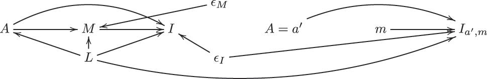
DAG of a twin network causal model with a mediator that illustrates the first part of the sequential ignorability (17), namely, the conditional independence of I
a′,m
and A, given L;
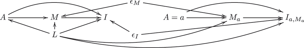
DAG of a twin network causal model with a mediator that illustrates the first part of the sequential ignorability (17), namely, the conditional independence of M
a
and A, given L;
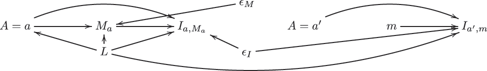
DAG of a twin network causal model with a mediator that illustrates the second part of the sequential ignorability (17), namely, the conditional independence of I
a′,m
and M
a
, given L and A=a;
A.2 Controlled direct effect NNT
Definition 4.
The marginal controlled direct effect (CDE) is defined as
where
However, since m is fixed, the inner conditional expectation
To express this difference in terms of observed data, we use the consistency assumption: I=I
a,m
when A=a and M=m, and the conditional ignorability assumption, i.e.,
therefore,
These quantities can be estimated using standard regression techniques. Applying the function g to p c (m) yields the controlled direct effect on the NNT scale, also interpretable as the NNT conditional on M=m. An analogous definition holds for the group-specific controlled direct effect:
For additional details and applications of this framework, see Refs. [17], 54]. As a final note, unlike other effect types, there is no corresponding “controlled indirect effect,” so we do not pursue this direction further.
A.3 Proof of Proposition 1
Proof.
The NIE is defined as
The first equality applies the law of total expectation. The second equality uses the fact that for M
1=M
0, the term
which concludes the proof. □
A.4 Proof of Proposition 2
Proof.
The NDE is defined as
where the last equality assumes
A.5 Identification of the indirect effect in the ath group
Although the illustration below focuses on the unexposed group A=0, the derivation for the exposed group A=1 is entirely analogous, with all expectations conditioned on A=1 instead. For the INNE, which is defined as g(p
i
(0)), we show the identification procedure for the first multiplicative term of eq. (12). Therefore, we need to express
The derivation for the second multiplicative term in eq. (12) follows the same steps for the conditional outcome model. Namely, assuming a conditional outcome model as in eq. (25),
Therefore, the indirect effect for the unexposed group p i (0; θ) is identified by
where θ denotes the set of all unknown parameters that the indirect effect is dependent on. Finally, the INNE is identified by g(p i (0; θ)). Replacing the conditioning set with A=1, that is, evaluating the expectations with respect to the exposed group, yields the identification formula for the indirect effect among the exposed group p i (1; θ), and consequently for the IEIN, defined as g(p i (1; θ)).
References
1. Nguyen, TQ, Schmid, I, Stuart, EA. Clarifying causal mediation analysis for the applied researcher: defining effects based on what we want to learn. Psychol Methods 2021;26:255. https://doi.org/10.1037/met0000299.Suche in Google Scholar
2. Rijnhart, JJM, Lamp, SJ, Valente, MJ, MacKinnon, DP, Twisk, JWR, Heymans, MW. Mediation analysis methods used in observational research: a scoping review and recommendations. BMC Med Res Methodol 2021;21:1–7. https://doi.org/10.1186/s12874-021-01426-3.Suche in Google Scholar
3. MacKinnon, DP, Lockwood, CM, Hoffman, JM, West, SG, Sheets, V. A comparison of methods to test mediation and other intervening variable effects. Psychol Methods 2002;7:83. https://doi.org/10.1037//1082-989x.7.1.83.Suche in Google Scholar
4. Preacher, KJ, Kelley, K. Effect size measures for mediation models: quantitative strategies for communicating indirect effects. Psychol Methods 2011;16:93. https://doi.org/10.1037/a0022658.Suche in Google Scholar
5. Lange, T, Starkopf, L. Commentary: mediation analyses in the real world. Epidemiology 2016;27:677–81. https://doi.org/10.1097/ede.0000000000000518.Suche in Google Scholar
6. Ditlevsen, S, Christensen, U, Lynch, J, Damsgaard, MT, Keiding, N. The mediation proportion: a structural equation approach for estimating the proportion of exposure effect on outcome explained by an intermediate variable. Epidemiology 2005:114–20. https://doi.org/10.1097/01.ede.0000147107.76079.07.Suche in Google Scholar
7. Newcombe, RG. Confidence intervals for proportions and related measures of effect size. Boca Raton, Florida: CRC Press; 2012.10.1201/b12670Suche in Google Scholar
8. Vancak, V, Goldberg, Y, Levine, SZ. Guidelines to understand and compute the number needed to treat. BMJ Ment Health 2021;24:131–6. https://doi.org/10.1136/ebmental-2020-300232.Suche in Google Scholar
9. Lee, TY, Kuo, S, Yang, CY, Ou, HT. Cost-effectiveness of long-acting insulin analogues vs intermediate/long-acting human insulin for type 1 diabetes: a population-based cohort followed over 10 years. Br J Clin Pharmacol 2020;86:852–60. https://doi.org/10.1111/bcp.14188.Suche in Google Scholar
10. Verbeek, JGE, Atema, V, Mewes, JC, van Leeuwen, M, Oldenburg, HSA, van Beurden, M, et al.. Cost-utility, cost-effectiveness, and budget impact of internet-based cognitive behavioral therapy for breast cancer survivors with treatment-induced menopausal symptoms. Breast Cancer Res Treat 2019;178:573–85. https://doi.org/10.1007/s10549-019-05410-w.Suche in Google Scholar
11. da Costa, BR, Rutjes, AWS, Johnston, BC, Reichenbach, S, Nüesch, E, Tonia, T, et al.. Methods to convert continuous outcomes into odds ratios of treatment response and numbers needed to treat: meta-epidemiological study. Int J Epidemiol 2012;41:1445–59. https://doi.org/10.1093/ije/dys124.Suche in Google Scholar
12. Mendes, D, Alves, C, Batel-Marques, F. Number needed to treat (nnt) in clinical literature: an appraisal. BMC Med 2017;15:1–13. https://doi.org/10.1186/s12916-017-0875-8.Suche in Google Scholar
13. Bender, R, Blettner, M. Calculating the “number needed to be exposed” with adjustment for confounding variables in epidemiological studies. J Clin Epidemiol 2002;55:525–30. https://doi.org/10.1016/s0895-4356(01)00510-8.Suche in Google Scholar
14. Laupacis, A, Sackett, DL, Roberts, RS. An assessment of clinically useful measures of the consequences of treatment. N Engl J Med 1988;318:1728–33. https://doi.org/10.1056/nejm198806303182605.Suche in Google Scholar
15. Kristiansen, IS, Gyrd-Hansen, D, Nexøe, J, Nielsen, JB. Number needed to treat: easily understood and intuitively meaningful? Theoretical considerations and a randomized trial. J Clin Epidemiol 2002;55:888–92. https://doi.org/10.1016/s0895-4356(02)00432-8.Suche in Google Scholar
16. Mueller, S, Pearl, J. Personalized decision making–a conceptual introduction. J Causal Inference 2023;11:20220050. https://doi.org/10.1515/jci-2022-0050.Suche in Google Scholar
17. Vancak, V, Sjölander, A. Estimation of the number needed to treat, the number needed to be exposed, and the exposure impact number with instrumental variables. Epidemiol Methods 2024;13:20230034. https://doi.org/10.1515/em-2023-0034.Suche in Google Scholar
18. Vancak, V, Goldberg, Y, Levine, SZ. Systematic analysis of the number needed to treat. Stat Methods Med Res 2020;29:2393–410. https://doi.org/10.1177/0962280219890635.Suche in Google Scholar
19. Kraemer, HC, Kupfer, DJ. Size of treatment effects and their importance to clinical research and practice. Biol Psychiatry 2006;59:990–6. https://doi.org/10.1016/j.biopsych.2005.09.014.Suche in Google Scholar
20. Grieve, AP. The number needed to treat: a useful clinical measure or a case of the emperor’s new clothes? Pharm Stat J Appl Stat Pharm Ind 2003;2:87–102. https://doi.org/10.1002/pst.33.Suche in Google Scholar
21. Hutton, JL. Number needed to treat: properties and problems. J Roy Stat Soc Ser A (Stat Soc) 2000;163:381–402. https://doi.org/10.1111/1467-985x.00175.Suche in Google Scholar
22. Snapinn, S, Jiang, Q. On the clinical meaningfulness of a treatment’s effect on a time-to-event variable. Stat Med 2011;30:2341–8. https://doi.org/10.1002/sim.4256.Suche in Google Scholar
23. Kristiansen, IS, Gyrd-Hansen, D. Cost-effectiveness analysis based on the number-needed-to-treat: common sense or non-sense? Health Econ 2004;13:9–19. https://doi.org/10.1002/hec.797.Suche in Google Scholar
24. Breitborde, NJK, Srihari, VH, Pollard, JM, Addington, DN, Woods, SW. Mediators and moderators in early intervention research. Early Interv Psychiatry 2010;4:143–52. https://doi.org/10.1111/j.1751-7893.2010.00177.x.Suche in Google Scholar
25. Tsai, CL, Camargo, CAJr. Methodological considerations, such as directed acyclic graphs, for studying “acute on chronic” disease epidemiology: chronic obstructive pulmonary disease example. J Clin Epidemiol 2009;62:982–90. https://doi.org/10.1016/j.jclinepi.2008.10.005.Suche in Google Scholar
26. Du Toit, G, Foong, RXM, Lack, G. Prevention of food allergy-early dietary interventions. Allergol Int 2016;65:370–7. https://doi.org/10.1016/j.alit.2016.08.001.Suche in Google Scholar
27. Carr, A. Cardiovascular risk factors in hiv-infected patients. JAIDS J Acquir Immune Defic Syndr 2003;34:S73–8. https://doi.org/10.1097/00126334-200309011-00011.Suche in Google Scholar
28. Pellegrini, V, De Cristofaro, V, Salvati, M, Giacomantonio, M, Leone, L. Social exclusion and anti-immigration attitudes in Europe: the mediating role of interpersonal trust. Soc Indic Res 2021;155:697–724. https://doi.org/10.1007/s11205-021-02618-6.Suche in Google Scholar
29. Rubin, DB. Causal inference using potential outcomes: design, modeling, decisions. J Am Stat Assoc 2005;100:322–31. https://doi.org/10.1198/016214504000001880.Suche in Google Scholar
30. Pearl, J. The causal mediation formula – a guide to the assessment of pathways and mechanisms. Prev Sci 2012;13:426–36. https://doi.org/10.1007/s11121-011-0270-1.Suche in Google Scholar
31. Forastiere, L, Mattei, A, Ding, P. Principal ignorability in mediation analysis: through and beyond sequential ignorability. Biometrika 2018;105:979–86. https://doi.org/10.1093/biomet/asy053.Suche in Google Scholar
32. Robins, JM, Greenland, S. Identifiability and exchangeability for direct and indirect effects. Epidemiology 1992;3:143–55. https://doi.org/10.1097/00001648-199203000-00013.Suche in Google Scholar
33. Docquier, F, Rapoport, H. Globalization, brain drain, and development. J Econ Lit 2012;50:681–730. https://doi.org/10.1257/jel.50.3.681.Suche in Google Scholar
34. Beine, M, Docquier, F, Rapoport, H. Brain drain and economic growth: theory and evidence. J Dev Econ 2001;64:275–89. https://doi.org/10.1016/s0304-3878(00)00133-4.Suche in Google Scholar
35. Beine, M, Docquier, F, Rapoport, H. Brain drain and human capital formation in developing countries: winners and losers. Econ J 2008;118:631–52. https://doi.org/10.1111/j.1468-0297.2008.02135.x.Suche in Google Scholar
36. Holland, PW. Statistics and causal inference. J Am Stat Assoc 1986;81:945–60. https://doi.org/10.2307/2289064.Suche in Google Scholar
37. Rubin, DB. Estimating causal effects of treatments in randomized and nonrandomized studies. J Educ Psychol 1974;66:688. https://doi.org/10.1037/h0037350.Suche in Google Scholar
38. Pearl, J. On the consistency rule in causal inference: axiom, definition, assumption, or theorem? Epidemiology 2010;21:872–5. https://doi.org/10.1097/ede.0b013e3181f5d3fd.Suche in Google Scholar
39. Petersen, ML, Porter, KE, Gruber, S, Wang, Y, Van Der Laan, MJ. Diagnosing and responding to violations in the positivity assumption. Stat Methods Med Res 2012;21:31–54. https://doi.org/10.1177/0962280210386207.Suche in Google Scholar
40. Imai, K, Keele L, Yamamoto T. Identification, inference and sensitivity analysis for causal mediation effects. Statistical Science 2010;25:51–71. https://doi.org/10.1214/10-sts321.Suche in Google Scholar
41. Imai, K, Keele, L, Tingley, D. A general approach to causal mediation analysis. Psychol Methods 2010;15:309. https://doi.org/10.1037/a0020761.Suche in Google Scholar
42. Frangakis, CE, Rubin, DB. Principal stratification in causal inference. Biometrics 2002;58:21–9. https://doi.org/10.1111/j.0006-341x.2002.00021.x.Suche in Google Scholar
43. Ding, P, Lu, J. Principal stratification analysis using principal scores. J Roy Stat Soc B Stat Methodol 2017;79:757–77. https://doi.org/10.1111/rssb.12191.Suche in Google Scholar
44. Cole, SR, Frangakis, CE. The consistency statement in causal inference: a definition or an assumption? Epidemiology 2009;20:3–5. https://doi.org/10.1097/ede.0b013e31818ef366.Suche in Google Scholar
45. Sjölander, A. Estimation of causal effect measures with the r-package stdreg. Eur J Epidemiol 2018;33:847–58. https://doi.org/10.1007/s10654-018-0375-y.Suche in Google Scholar
46. Bender, R, Kuss, O, Hildebrandt, M, Gehrmann, U. Estimating adjusted NNT measures in logistic regression analysis. Stat Med 2007;26:5586–95. https://doi.org/10.1002/sim.3061.Suche in Google Scholar
47. Nevo, D, Liao, X, Spiegelman, D. Estimation and inference for the mediation proportion. Int J Biostat 2017;13:20170006. https://doi.org/10.1515/ijb-2017-0006.Suche in Google Scholar
48. Bender, R, Vervölgyi, V. Estimating adjusted nnts in randomised controlled trials with binary outcomes: a simulation study. Contemp Clin Trials 2010;31:498–505. https://doi.org/10.1016/j.cct.2010.07.005.Suche in Google Scholar
49. Stefanski, LA, Boos, DD. The calculus of m-estimation. Am Stat 2002;56:29–38. https://doi.org/10.1198/000313002753631330.Suche in Google Scholar
50. VanderWeele, TJ. Bias formulas for sensitivity analysis for direct and indirect effects. Epidemiology 2010;21:540–51. https://doi.org/10.1097/ede.0b013e3181df191c.Suche in Google Scholar
51. Valeri, L, VanderWeele, TJ. Mediation analysis allowing for exposure–mediator interactions and causal interpretation: theoretical assumptions and implementation with sas and spss macros. Psychol Methods 2013;18:137. https://doi.org/10.1037/a0031034.Suche in Google Scholar
52. Balke, A, Pearl J. Probabilistic evaluation of counterfactual queries. In: Probabilistic and causal inference: the works of Judea Pearl. New York, NY, USA: Association for Computing Machinery; 2022:237–54 pp.10.1145/3501714.3501733Suche in Google Scholar
53. Pearl, J. Causality. Cambridge, UK: Cambridge University Press; 2009.Suche in Google Scholar
54. Vancak, V, Goldberg, Y, Levine, SZ. The number needed to treat adjusted for explanatory variables in regression and survival analysis: theory and application. Stat Med 2022;41:3299–320. https://doi.org/10.1002/sim.9418.Suche in Google Scholar
55. Pearl, J. Direct and indirect effects. In: Probabilistic and causal inference: the works of Judea Pearl. New York, NY, USA: Association for Computing Machinery; 2022:373–392 pp.10.1145/3501714.3501736Suche in Google Scholar
© 2025 Walter de Gruyter GmbH, Berlin/Boston
Artikel in diesem Heft
- Research Articles
- Definition, identification, and estimation of the direct and indirect number needed to treat
- Sample size determination for external validation of risk models with binary outcomes using the area under the ROC curve
- Analysis of the drug resistance level of malaria disease: a fractional-order model
- Extending the scope of the capture-recapture experiment: a multilevel approach with random effects to provide reliable estimates at national level
- Discrete-time compartmental models with partially observed data: a comparison among frequentist and Bayesian approaches for addressing likelihood intractability
- Sensitivity analysis for unmeasured confounding for a joint effect with an application to survey data
- Investigating the association between school substance programs and student substance use: accounting for informative cluster size
- The quantiles of extreme differences matrix for evaluating discriminant validity
- Finite-sample improved confidence intervals based on the estimating equation theory for the modified Poisson and least-squares regressions
- Causal mediation analysis for difference-in-difference design and panel data
- What if dependent causes of death were independent?
- Bot invasion: protecting the integrity of online surveys against spamming
- A study of a stochastic model and extinction phenomenon of meningitis epidemic
- Understanding the impact of media and latency in information response on the disease propagation: a mathematical model and analysis
- Time-varying reproductive number estimation for practical application in structured populations
- Perspective
- Should we still use pointwise confidence intervals for the Kaplan–Meier estimator?
- Leveraging data from multiple sources in epidemiologic research: transportability, dynamic borrowing, external controls, and beyond
- Regression calibration for time-to-event outcomes: mitigating bias due to measurement error in real-world endpoints