
Frequency response locking of electromagnetic vibration-based energy harvesters using a switch with tuned duty cycle
-
Aboozar Dezhara


Abstract
It is proposed to tune linear electromagnetic vibration-based energy harvesters so that they will achieve an optimum case regardless of the base amplitude or excitation frequency of the environment. The author designed the optimum coil and load parameters as well as the optimum acceleration amplitude and vibration frequency of the magnet for known values of three mechanical parameters (spring constant, mass, and mechanical damping coefficient) so that the optimum parameters will remain constant upon switching. As the vibration frequency of the magnet deviates from the optimal value, the switch turns on and off to compensate for the deviation so that the maximum power entering the electrical domain does not change. The deviation is limited to frequency or base amplitude acceleration. Other optimum parameters are fixed values. They are designed so that they can handle the maximum power that is delivered to the electrical domain.
Introduction
There is an increasing interest in making sensors to be self-contained with their renewable power supply in order to maximize the performance of these devices (Ottman et al. 2002). Moreover, recent developments in microelectronics technology have reduced the power requirements of these electronics and wearable/implantable devices to milliwats (Dong et al. 2019). Thus, it is becoming increasingly possible to implement self-power from non-conventional sources. An effective linear electromagnetic vibration-based energy harvester (EVEH) converts mechanical vibrations to electrical power when the ambient excitation frequency matches the specific resonant frequency of the device (Lee and Chung 2015). It should be note that this resonance frequency depends on not only spring constant and mass of the magnet but also on the electrical parameters of electrical domain and electromagnetic coupling coefficient. There are many authors that use the broadening of bandwidth approach through many methods (Aboulfotoh, Arafa, and Megahed 2013; Berdy et al., 2011; Chen, Wu, and Liu 2014; Jung and Seok 2015; Lee and Chung 2015). Generally these methods alter the intrinsic parameters that resonance frequency depends on them, such as spring constant or mass of magnet somehow to match the resonance frequency of harvester with excitation frequency of environment also these author generally doesn’t consider the effect of electrical parameters on resonance frequency. Nevertheless, the author consider it in this paper. But this method of tuning dose not very much contribute to improving performance because the peak of frequency response will decrease significantly at not very far from mechanical resonance frequency. The researchers refer to nonlinear spring to broaden the bandwidth of harvester and solve this problem, but the nonlinear spring increase the complexity and brings up higher harmonics. In our tuning method we did not alter the mass or spring, but tune the system so that the magnet always vibrates at optimum vibration frequency, regardless of the excitation frequency of environment or base amplitude acceleration. In “Basic principles of EVEH” section of this paper the basic principles of EVEH is introduced, the main section of this paper is “Transfer function and duty cycle” section where the analysis of switching circuit and derivation of transfer function and as a result, derivation of electrical damping coefficient for three kind of load and how to derive duty cycle are elaborately discussed. In “Coil parameters design and numerical example” section the calculation of optimum parameters values such as vibration frequency of magnet and base amplitude acceleration are discussed. The remaining two section i.e. “Discussion” and “Conclusion” sections of seven and eight are impedance matching and how to derive power as well as damping for plotting of frequency response are discussed.
Basic principles of EVEH
Faraday’s law of induction
This law can be formulated as follows:
where K, z, φ, VEMF are electromagnetic coupling coefficient, displacement of mass (moving magnet) relative to the case, flux of magnetic field that pass from the coil, the turns of the coil and induced voltage in the coil respectively. The dot shows differential with respect to time. It should be note that the coil is fixed with respect to the case and the electromagnetic coupling coefficient just depends on the geometry of the magnet (mass) and flux linkage between the magnet and the coil, the calculation of K is beyond the scope of our work and in this paper we assume it is given and constant.
Equation of vibration of EVEH
According to the second law of newton in mechanic (Chen, Wu, and Liu 2014):
where m, Cm, ks, FEM, y are mass of the moving magnet, mechanical damping coefficient, constant of spring, electrical damping force imposed on the magnet, and input excitation displacement respectively. It should be noted that this is the magnetic drag force i.e. FEM that play role in producing an electrical current in the coil. We should someway relate this force to the electrical current. We proceed as follows:
If we equate the generated electrical power in the coil to the power of the force FEM we can relate this force to the electrical current:
From equations (3) and (4) we conclude that:
Equation (5) tell us that the electromagnetic force have linear relationship with the electrical current that generated in the coil of energy harvester. This relation is consistent with the force implied on the conductor carrying current in magnetic field:
The proportionality factor is called electromagnetic coupling coefficient. The larger this factor the more flux linkage we have. The second relation also tell us that the electromotive force has relationship with velocity.
Transfer function and duty cycle
In this section the transfer function and formulas for calculating the suitable duty cycle will derived at general electrical loads.
Resistive load
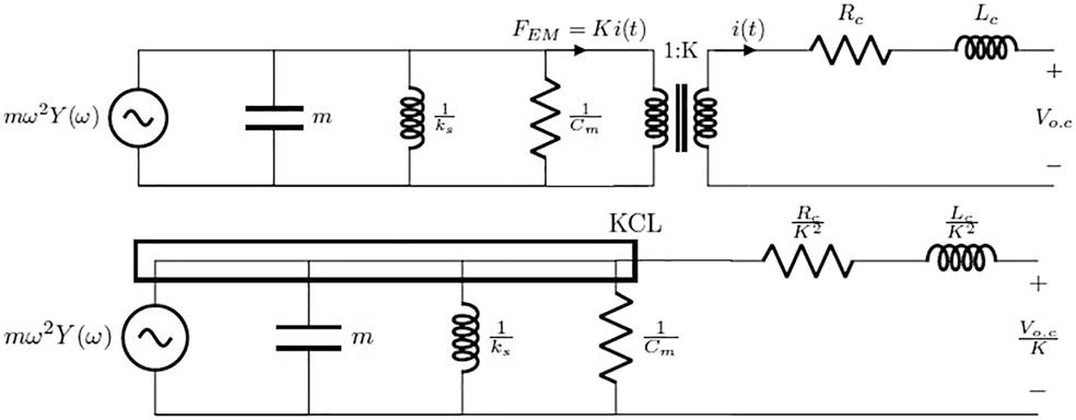
We can put equation (2) in frequency domain (Figure 1).
where ω is excitation frequency and we assume
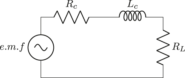
Electrical side of EVEH for resistive load.
If we write
By factoring
By equaling the real part of transfer function denominator to zero the resonance condition will be derived:
We will use this equation along with (5) other equation (that will be derived in “Coil parameters design and numerical example” section of this paper) to designing the coil and load parameters that are able to withstand the maximum power. It should be noted from equation (14) that if you neglect the first term in this expression, then the vibration frequency of magnet will be identical to the mechanical resonance frequency. But what is exactly the first (new) term in equation (14)? We can write equation (14) in the following form:
where the
Switching circuit for resistive load
The Kirchhoff current law (KCL) equation is (Figure 2):

Switching circuit of resistive load.
The next step is to analyze the load current and voltage waveforms and determine the root mean square (RMS) relations of voltage and current. Note that the switch start on and off when the magnet vibrates at off-optimum frequency as a result of off-optimum excitation frequency or at other words as a result of deviation from optimum base amplitude acceleration. These optimum parameters such as base amplitude acceleration, vibration frequency of magnet, coil parameters, etc. are as many as six and the author will discuss them in “Coil parameters design and numerical example” section. Note that the values of
The voltage and current waveform are not exactly sinusoidal, but the current value when the switch is on follows the equation of 18. The simplified equation (20) is as follows:
where
After simplification of equation (26) we have:
where
If we put the Vrms and Irms in (17) and squaring both sides and arrange and square again we have:
where
Note that in these equations we have two unknown variable, Ts and k. The value of Ts should be given and is a constant, the upper bound in sum formulas (p) depend on Ts and does not allow to solve simultaneously for k and Ts. However we can solve for k and λ from Kirchhoff current law (KCL) i.e. equation (17) and power condition (that will be discussed in more detail in this section). The equation (30) is a constraint equation. Note that the numerator of equation (29) is always zero so that the denumerator became A = B. This condition in addition of the formula that will drive from power condition result in the two unknown variables k and λ. In solving the numerical example, the parameter Ts should be given because of the reason mentioned above. We equate the output power from the switching circuit to the optimum power that is the best case of maximum power that can be harvested. The resulting formula in addition to formula derived from KCL (condition A = B) and the constrained relation from λ definition (equation (30)) can help us to solving the value of duty cycle.
Equation (32), and the condition of A = B as well as the formula of (30) can be solved simultaneously at given Ts to obtain the parameters of k (duty cycle).
Capacitive load
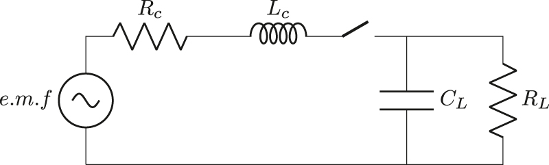
We can write the circuit equation of energy harvester with capacitive load as follows (Figure 3):
where VL is load voltage and CL is the load capacitor and I is the coil current. If we put equation (33) into frequency domain we will have:

Electrical side of EVEH for capacitive load.
Now we should someway obtain the
If we put equation (34) into equation (36) and solve for
If we put
The electrical damping coefficient and resonance condition of EVEH can be calculated by arranging the imaginary and real part of the denumerator of relation (38) respectively.
The resonance condition is:
Switching circuit for capacitive load
The RMS of load voltage can be derived using the derivative of equation (24) (Figure 4):
Switching circuit of capacitive load.
By similar way we have:
The parameter B is the same parameter as derived in previous subsection. According to KCL equation we have:
If we put equations (21), (27), (42) into equation (43) and after squaring the left and right side, arrange and square again we have:
where
Equation (27) have been used for Vrms. If we equate the formulas of equation (46) a relation for k will be derived. The switching waveforms are assumed to exactly coincide with sinusoidal curves of optimum condition voltage and current at times when the switch is on and the excitation frequency is optimum.
Two equations (44) and (47) can be numerical solved for k in MATLAB.
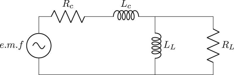
Electrical side of EVEH for inductive load.
Inductive load
When we put equation (48) into frequency domain, we get the following (Figure 5):
LL is the load inductance and IL is the inductor current, and here are the circuit equations:
Equation (49) into equation (51):
Solve for
In order to determine the electrical damping coefficient, factor out the term
By considering the real part of the denominator of equation (53), the resonance condition for EVEH at inductive load is:
Switching circuit for inductive load
Based on the KCL equation in the load node, we have (Figure 6):
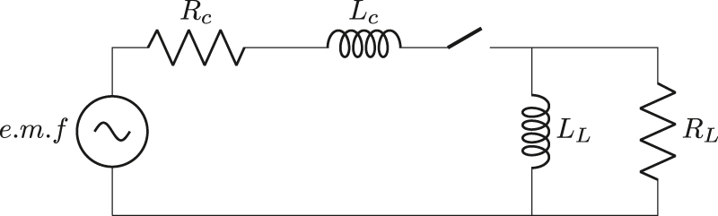
Switching circuit of inductive load.
Integration from equation (24) results in equation (57) and putting this equation and equations (21), (27) into equation (56), square the left and right sides arrange and square again, we have:
where
The values of A and B are the same as those found in equations (22), (28) respectively. To solve for k at the known value of Ts we need another equation that comes from power formula. This equation is exactly the same as equation (47).
4 Coil parameters design and numerical example
In our tuning problem, no matter what the excitation frequency or Ab is (just the value of excitation amplitude is a given and is a fixed value), we tune the frequency of vibration of the magnet so that the magnet vibrates regardless of the excitation frequency. When the excitation frequency changes, the base amplitude acceleration will change. The switching action brings the magnet from an off-optimum condition (i.e. different ω) to an optimum condition that will be discussed in the following. In this section, we will use six equations that will help us to design coil and load parameters that are able to withstand under-input power that enters the electrical domain of EVEH. These six equations include resonance condition as well as power (that delivered to the electrical domain) derivative with respect to the angular frequency of magnet at constant load and constant base amplitude acceleration, and power (that consumed in the load resistor) derivative with respect to load at a constant angular vibration frequency of magnet and constant base amplitude acceleration which results to third and fourth equations and the load that derived from this derivative is equivalent to Thévénin-based load that will drive in “Impedance matching” section (relations of 85 and 90 for the case of capacitive load). The fifth equation is derived through the derivative of power that entered into the electrical domain with respect to the electrical damping coefficient and the sixth equation is derived through the formula of
This is the first equation of the three mentioned above conditions. The second equation is obtained by equating the derivative of the real part of the power that is delivered to the electrical domain with respect to angular frequency to zero. As mentioned above the third and fourth equations are equivalent to the Thévénin-based load parameters. The fifth and sixth conditions are derived as follows: maximum active root mean square (RMS) power that will deliver to the electrical part is:
Applying the resonance conditions to the transfer function, we get:
Therefore
This is the fifth equation. The sixth relation is the formula of base amplitude acceleration i.e.
If we place the 67 condition into the power transferred to the electrical domain i.e. equation (65), we get:
Equation (68) shows that when the base acceleration is constant the maximum power delivered to the electrical domain is constant, and this formula does not depend on the electromagnetic coupling coefficient. The smaller the mechanical damping the more energy will be delivered to the electrical domain. Note that Pmax is a RMS power.
Capacitive load numerical example
In this subsection, the author will show that Thévénin-based load parameters, as well as other optimum parameters such as Ab, ω (vibration frequency of magnet), and coil parameters, can be calculated using MATLAB based on six equations discussed above. Note that if the coil and load are able to withstand these optimum Ab and ω, then they can be able to withstand other Ab and ω. It should be noted that the inductive nature of the system at Micro or Nano dimension does not allow applying the inductive load for locking the frequency response, because (based on the Table 3 that will be explained in “Discussion” section) the intermittent environment (i.e. the coil) is also inductive. Therefore, the balancing process of reactive energies becomes more improbable. Nevertheless, the theoretical analysis and discussion of inductive load have been mentioned in this paper. The optimum parameters that cause the maximum electrical power to enter into that electrical domain based on the six equations discussed above are shown in Table 1. According to our tuning strategy, we want EVEH to operate in these optimum parameters regardless of the base amplitude acceleration or excitation frequency of the environment. When the base amplitude acceleration changes and deviates from the optimum value the vibration frequency of the magnet will also tend to change and as a result of this, we cannot achieve the optimum power in the load resister, to overcome this deviation we apply a switch between coil and load and tune the duty cycle of this switch so that we are able to achieve the optimum power in optimum load resistor. To calculate the deviated vibration frequency of the magnet whenever the base amplitude changes from the optimum condition, the base amplitude acceleration formula (
The optimum parameters of EVEH with known values of three mechanical parameters and given value of Y0 = 1e−4 (g = 9.81 m/s2).
| Symbol | Quantity | value | Unit |
|---|---|---|---|
| m | Mass of moving magnet | 21.4 | g |
| ks | Spring constant | 3220 | N/m |
| Cm | Mechanical damping | 0.31 | N s/m |
| K | Electromagnetic coupling | 5.6 | V s/m |
| Ab | Base acceleration | 1.427 g | m/s2 |
| Rc | Coil resistance | 28.53 | |
| Lc | Coil reactance | 1.168 | H |
| RL | Load resistance | 4.6240 | |
| CL | Load capacitance | 6.078 | |
| fexc | Excitation frequency | 59.56 | Hz |
Duty cycle for the different excitation frequency and for optimum parameters of
| Excitation frequency | Duty cycle | Switching frequency |
|---|---|---|
| fexc = 2 Hz | k = 0.1024 | fs = 150 Hz |
| fexc = 25 Hz | k = 0.1021 | fs = 150 Hz |
| fexc = 35 Hz | k = 0.7660 | fs = 150 Hz |
| fexc = 80 Hz | k = 0.0972 | fs = 150 Hz |
| fexc = 110 Hz | k = 0.4425 | fs = 150 Hz |
Note that 13.7 mW consumes in the resistor of the coil i.e. 37.85% of maximum power that enters into the electrical domain. These numbers tell us that with the optimum parameters of Table 1 we cannot harvest more than 22.5 mW at optimum load resistor and optimum excitation frequency. Note that according to our calculations (Table 2), at frequencies more than the optimum excitation frequency (i.e. 59.56 Hz), harvesting the optimum power using a switching circuit for capacitive load is not impossible.
Impedance matching
Thévénin circuit of EVEH
Based on the electrical similarity of mechanical systems (Cammarano et al. 2010) we can say:
A diagram of the EVEH circuit is shown in Figure 7. FEM is the electrical damping force and
where

The circuit model of EVEH.
Thévénin circuit for open circuit voltage.
If we put equation (73) into (71) (Figure 9):

Thévénin circuit of short circuit current.
After simplifying we have:
The condition of maximum power transfer
If the load impedance is equal to the conjugate of Thévénin impedance, then maximum power will be delivered from the source to the load (Berdy et al. 2011).
Resistive load
Note that in resistive load we assume the coil inductance is negligibly
Note that
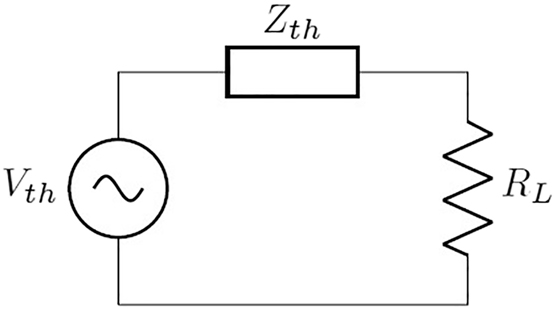
Thévénin equivalent circuit for resistive load.
Capacitive load
If we divide equation (83) by (82) (Figure 11):
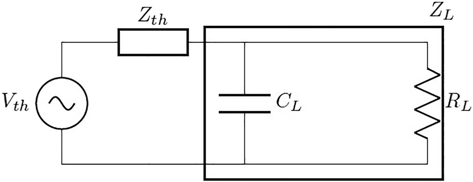
Thévénin equivalent circuit for capacitive load.
Assuming that we put equation (84) into equation (82) and arrange the result in terms of RL and put it in equation (84):
These equations are the optimum load formula for capacitive loads.
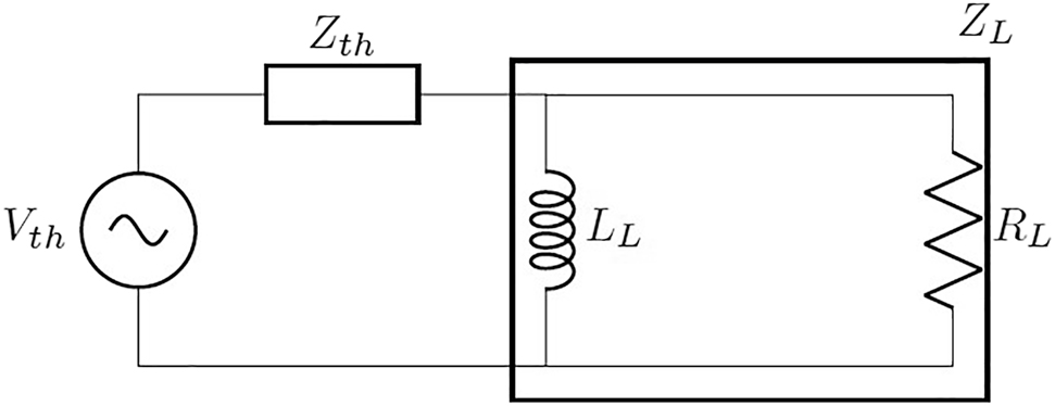
Thévénin equivalent circuit for inductive load.
Inductive load
If we divide equation (87) by (88) (Figure 12):
Putting equation (89) into equation (88) and simplifying:
These equations are the optimum load formula for inductive load this load is emulated by a switch with variable duty cycle.
Complex damping and RMS power formulas
In this section, we elaborate on how frequency response will be plotted as well as electrical damping coefficient and lock coefficient (imaginary part of complex damping).
Resistive load
The load voltage for resistive load is (equation (10)):
The power is the time derivative work of the electric damping force FEM:
We can calculate the power based on the generated electrical current. Inputting equation (9) into equation (93):
Putting equations (91) into (94), we can derive the power formula:
Based on the simplified equation above:
The standard form of this equation is:
The real part of equation (100) corresponds to the electrical damping, which is a factor that affects the mechanical damping coefficient. Reactive power may also be generated by the passive components of the circuit. Mass and spring also store reactive power. It’s easy to conclude that the real part of equation (97) is energy generated in a coil and load resistors, the imaginary part refers to the reactive energy generated in the coil’s inductor. The resistor RL consumes the following amount of power:
The amount of reactive power generated in the coil is:
As
Capacitive load
According to “Capacitive load” section, the load voltage for capacitive load can be derived from equation (37).
The voltage across the load resistor is represented by the above equation. The following happens if we plug equation (105) into equation (34):
Since we know the value of load current, we can calculate the integral of equation (93):
In this equation Ce is equal to equation (100), where
In order to distinguish real power generated in Rc and RL from reactive power generated in Lc and CL, we first calculate the real part of equation (107):
The real power is the sum of power that is generated in the coil and in the load resistors. We can distinguish between these two powers, i.e.
Subtracting equation (112) from equation (110) we find the power consumed by the resistor of the load (i.e.
The frequency-response plot is the plot of
The generated current passes the Lc is known, we can calculate the reactive power generated by the Lc as follows:
where
As a result, if we subtract equation (116) from equation (114), the reactive power consumed by the load capacitor will be as follows:
Knowing transfer function for capacitive load, we can plot voltage and power versus frequency from equations (105) and (113).
Inductive load
If we put equation (118) into (49) the current will be derived:
Putting equation (119) into equation (7), the following power will be derived:
The formula for ce is the same as equation (100).
Here is the real part of the equation:
As a result of subtracting equation (125) from equation (123):
Inductive loads are described by equation (126) for
The generated reactive power,
By knowing the transfer function for an inductive load, we can plot voltage and power versus frequency from equations (118) and (126).
Discussion
In this paper, we proposed a switch to lock the frequency response of EVEH. However, we did not discuss how the switch operates. Considering the resonance condition, we can write it as follows for each of the loads mentioned above.
Multiply the left side by
Reactive energy balance for the whole system is described by (133):
where Ek is the kinetic energy of magnet and
The loads that should be applied in various conditions.
| Frequency | Thévénin reactance | Applied load |
|---|---|---|
| R−C | ||
| R−L | ||
| R−C | ||
| R−L |
Conclusions
Therefore, we have shown how we can use a switch with a specific switching frequency and duty cycle that depends just on the off-optimum vibration frequency of the magnet, to lock the frequency response of EVEH so that the optimum parameters are always guaranteed. The only issue is the mode of operation of the switch in our analysis, which with reactive elements of energy such as mass and spring, it is guaranteed that no net reactive energy remains in the system after the switch turns on and off.
-
Author contributions: All the authors have accepted responsibility for the entire content of this submitted manuscript and approved submission.
-
Research funding: None declared.
-
Conflict of interest statement: The authors declare no conflicts of interest regarding this article.
References
Aboulfotoh, N., M. Arafa, and S. Megahed. 2013. “A Self-Tuning Resonator for Vibration Energy Harvesting.” Sensors and Actuators A Physical 210: 328–34.10.1016/j.sna.2013.07.030Suche in Google Scholar
Berdy, D., B. Jung, J. Rhoads, and D. Peroulis. “Increased-Bandwidth, Meandering Vibration Energy Harvester.” In 2011 16th International Solid-State Sensors, Actuators and Microsystems Conference, TRANSDUCERS’11, 06, 2011.10.1109/TRANSDUCERS.2011.5969872Suche in Google Scholar
Chen, S., J. Wu, and S. Liu. 2014. “Electromagnetic Energy Harvester with an In-Phase Vibration Bandwidth Broadening Technique.” In 2014 IEEE 27th International Conference on Micro Electro Mechanical Systems (MEMS), 382–4.10.1109/MEMSYS.2014.6765656Suche in Google Scholar
Cammarano, A., S. G. Burrow, D. Barton, A. Carrella, and L. Clare. 2010. “Tuning a Resonant Energy Harvester Using a Generalized Electrical Load.” Smart Materials and Structures 19: 055003.10.1088/0964-1726/19/5/055003Suche in Google Scholar
Dong, L., A. Closson, C. Jin, I. Trase, Zi. Chen, and X. Zhang. 2019. “Vibration-Energy-Harvesting System: Transduction Mechanisms, Frequency Tuning Techniques, and Biomechanical Applications.” Advanced Materials Technologies 4: 08, https://doi.org/10.1002/admt.201900177.Suche in Google Scholar PubMed PubMed Central
Jung, J., and J. Seok. 06 2015. “Frequency-tunable Electromagnetic Energy Harvester Using Magneto-Rheological Elastomer.” Journal of Intelligent Material Systems and Structures 27: 959–79.10.1177/1045389X15590274Suche in Google Scholar
Lee, B., and G. Chung. 2015. “Frequency Tuning Design for Vibration-Driven Electromagnetic Energy Harvester.” IET Renewable Power Generation 9 (7): 801–8, https://doi.org/10.1049/iet-rpg.2014.0195.Suche in Google Scholar
Ottman, G. K., H. F. Hofmann, A. C. Bhatt, and G. A. Lesieutre. 2002. “Adaptive Piezoelectric Energy Harvesting Circuit for Wireless Remote Power Supply.” IEEE Transactions on Power Electronics 17 (5): 669–76, https://doi.org/10.1109/tpel.2002.802194.Suche in Google Scholar
© 2022 Walter de Gruyter GmbH, Berlin/Boston
Artikel in diesem Heft
- Frontmatter
- Research Articles
- Optimized routing with efficient energy transmission using Seline Trustworthy optimization for waste management in the smart cities
- Effectiveness of line type and cross type piezoelectric patches on active vibration control of a flexible rectangular plate
- Energy visibility of a modeled photovoltaic/diesel generator set connected to the grid
- Techno-economic analysis and design of hybrid renewable energy microgrid for rural electrification
- The comparison of triboelectric power generated by electron-donating polymers KAPTON and PDMS in contact with PET polymer
- Investigation of aerodynamic interaction between the balloon and the ducted wind turbine in airborne configuration
- Experimental investigation on treated transformer oil (TTO) and its diesel blends in the diesel engine
- Frequency response locking of electromagnetic vibration-based energy harvesters using a switch with tuned duty cycle
- Evaluation of energy generation in Iraqi territory by solar photovoltaic power plants with a capacity of 20 MW
- Review
- Quantitative analysis of DC–DC converter models: a statistical perspective based on solar photovoltaic power storage