Houses as Collateral and Household Debt Deleveraging in Korea
-
Joonhyuk Song


Abstract
As Korea’s household debt has increased rapidly since the mid-2000s, concerns that its economy’s hard-wired leveraging may negatively impact economic activity have grown. Calls are being made for policy actions to return the economy to its long-run trend. Housing preferences and monetary shocks can both trigger deleveraging, as most household debt is profoundly connected to the housing market, and debt growth increases sensitivity to interest rates. Constructing a dynamic stochastic general equilibrium model with heterogeneous households and the housing production sector, we simulate and analyze the macroeconomic effects of deleveraging. Because a lower loan-to-value (LTV) ceiling limits the size of household debt, the deleveraging effect caused by borrowers’ re-optimization is alleviated as the LTV ceiling decreases. When the housing price is included as an additional operating target in an otherwise standard monetary policy (MP) rule, economy-wide welfare increases when the MP is proactive to demand shocks and inactive to supply shocks. These findings suggest that deleveraging risk can be attenuated by adopting a lower LTV ceiling and maneuvering MP asymmetrically depending on the source of a shock.
1 Introduction
Korea is regarded as a leading and influential emerging economy and has unique real estate and housing markets characterized by the Chonsei system (Kim, Cho, & Ryu, 2018a, 2018b, 2019).[1] With potential buying pressure in the housing and asset markets and substantial borrowing demand due to Chonsei contracts,[2] Korea’s household debt started increasing in the early 2000s and has continuously accumulated over the last 20 years. Because this debt has grown too quickly in Korea and is highly concentrated in the housing market, concerns are growing that underperformance in the housing market will trigger a domino effect of household debt deleveraging. This outcome would heavily impact both the stability of the real economy and the financial system. Household debt deleveraging is recognized as the single most serious risk over the last several years. Policymakers are aware of the potential issues that may arise from deleveraging and continuously warn that the market must limit housing-related lending.
In Korea, the growth rates of household debt and household income move in opposite directions. Figure 1 shows that the household credit growth rate, which fell below 2% in 2003, rapidly rose up to almost 12% in 2006 owing to an overheated real estate market. It then declined following the introduction of the debt-to-income ratio. This growth rate has rebounded since 2012. Disposable income grew at an annual rate of about 6% through 2011, but this growth rate has dropped to 4% since 2012. As a result, the ratio of household credit to disposable income has steadily increased from 58.7% in 2003 to 82.2% in 2016, with the exception of a dip in 2004, as shown in Figure 2.
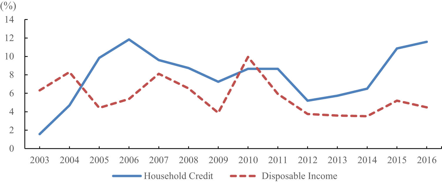
Growth rates of household credit and disposable income. Note: Household credit is composed of household loans and the sales credits of depositors and other financial institutions. Source: Bank of Korea.
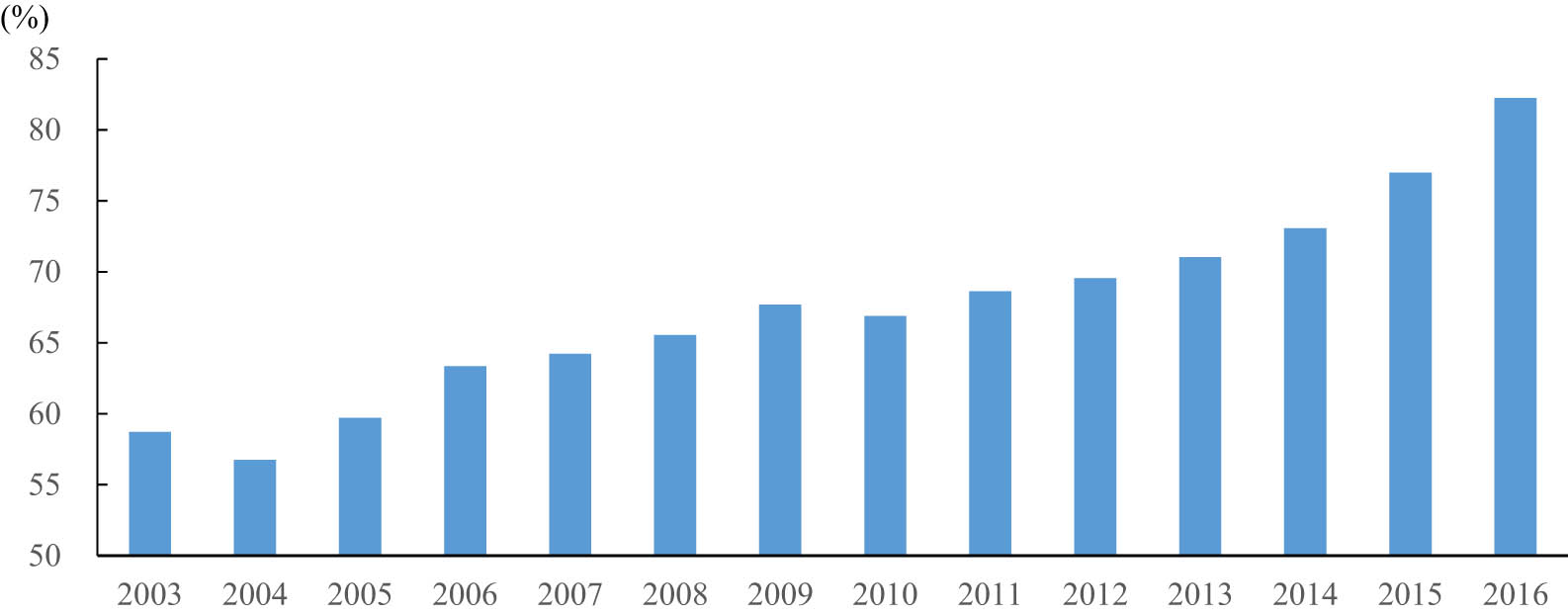
Ratio of household credit to disposable income. Source: Bank of Korea.
Household debt deleveraging refers to the phenomenon in which the credit supply suddenly shrinks and debt sharply falls as financial institutions cease lending or refuse revolving loans. This decrease in lending is caused by a decline in the collateral value of debt households when asset prices fall owing to shocks caused by tightened lending regulations, interest rate hikes, and so forth. If household debt deteriorates owing to a decline in real estate prices and a rise in interest rates, then both the loan-to-value (LTV) ratio and the financial burden from interest payments increase accordingly. Owing to the high level of outstanding debt, households become more sensitive to interest rates, and financial institutions grow more reluctant to provide new loans and refuse to revolve existing debts, as they need to meet the LTV ratio ceiling set by the supervising authority. As debt-ridden households sell their houses, housing prices decline and the LTV ratio deteriorates further, creating a vicious cycle.[3] When the government shifts to a policy of tightening to solve the household debt problem, the asset market collapses and the financial institutions’ credit supply shrinks, reducing the households’ capacity to repay their debts and leaving many households insolvent. This vicious cycle, known as debt deflation, not only aggravates the macroeconomy but also increases the financial risk. The financial intermediary function is also likely to deteriorate as credit supply falls.
In theory, household debt can play either a positive or negative role depending on the state of the economy. On the positive side, borrowing for consumption or asset purchases increases total consumption and construction investments (Di Maggio et al., 2017; Seppecher & Salle, 2015). On the negative side, an excessively high level of household debt can reduce GDP by restricting the consumption of borrowers, who must service their debts, and reducing investment, as higher debt levels increase interest rates (Benigno, Eggertsson, & Romei, 2020; Cecchetti & Kharroubi, 2012; Cecchetti, Mohanty, & Zampolli, 2011; Law & Singh, 2014; Mian, Sufi, & Verner, 2017). Taken together, household debt can positively affect GDP in the short term, but it becomes a burden on the economy once it reaches a certain threshold. If the household debt exceeds this threshold, the negative effects offset the positive effects and eventually dominate the economy.[4]
Academics and policymakers have recently reached a consensus that the Korean economy is approaching the threshold rapidly. The subsequent discussions focus on the timing, scope, and degree of the adverse effects of household debt and the introduction of policy measures to reduce the magnitudes of the negative impacts. Rising interest rates directly reduce consumption and investment, and the decline in lending to businesses and households due to asset price declines through financial accelerators further reduces consumption and investment. Importantly, these issues with household debt are related to the total debt stock rather than the increase or decrease in the stock at a particular time. An increase in interest rates affects not only newly issued debt but also the entire stock of outstanding debt (Cerutti & Claessens, 2017). When this stock is so large that households need to borrow more to pay the interest on their existing debts, the economy reaches a tipping point at which a flow problem becomes a stock problem. Thus, policies to keep the stock of debt from crossing this tipping point are the first line of defense to allow the economy to land softly during a deleveraging phase.
Previous studies on the relationships between the housing sector and economic variables can be divided into two categories: studies using vector autoregression (VAR) models and studies using dynamic stochastic general equilibrium (DSGE) models. Iacoviello (2005) presented a DSGE model with limited household borrowing up to a certain fraction of the house’s value, i.e., an LTV ceiling. Since this seminal work, follow-up studies have been continuously conducted. Iacoviello and Neri (2010) extended Iacoviello’s (2005) model to demonstrate the existence of spillover effects from the housing market to non-housing consumption. Guerrieri and Iacoviello (2017) solved a nonlinear version of Iacoviello’s (2005) model. In the Korean market, Song (2008) analyzed the effects of macroeconomic factors on domestic housing prices using a dynamic factor VAR model and reports that national factors explain 78% of the total volatility in housing prices. Lee and Song (2015) examined the relationship between real estate prices and key economic variables by constructing a DSGE model that includes the housing production sector, and they discuss the role of real estate in the Korean business cycle.
However, the previous DSGE models do not directly include real estate as an investment asset;[5] instead, they treat it as a type of collateral to alleviate borrowing limits. In other words, real estate is treated as a vehicle for smoothing consumption, and the models include no explicit explanations of how real estate is produced and traded in the market. This study, in contrast, includes housing in the DSGE model to examine its investment and collateral roles. We also include heterogeneous households to see how differences in preferences affect the transmission of policy shocks and examine the economic impacts of household debt deleveraging triggered by a decline in real estate prices. This study also treats housing construction as a separate production sector to allow the housing supply to respond to housing prices. When the housing supply is exogenously given, changes in housing prices affect the economy only through incomes, as the housing supply cannot respond to housing prices. Thus, by allowing the housing market to adjust for housing prices, we can analyze the interactions among consumption, non-housing investments, monetary policy (MP), and housing in more detail. From a modeling standpoint, we primarily follow Iacoviello and Neri (2010), assuming that households have heterogeneous desires to save and collateral constraints to capture housing business cycles. Whereas Iacoviello and Neri (2010) discussed the economic fluctuations caused by housing investments and production in an economy with heterogeneous households, this study focuses on the effectiveness of central bank MPs that set borrowing restrictions, such as LTV ceilings, in the housing sector. This study also discusses whether a housing-price-adjusted MP rule is more effective under demand- or supply-driven shocks, which Iacoviello and Neri (2010) and other previous studies do not address.
This study compares the macroeconomic effects of deleveraging for different LTV ratio requirements and, thus, is similar to previous studies on the contribution of the leveraging and deleveraging cycles to the US economy. In particular, Justiniano, Primiceri, and Tambalotti (2015) concluded that exogenous shifts in collateral requirements are not the main driver of macroeconomic outcomes, and they challenge the perspective that an exogenous tightening of collateral requirements was the main trigger of households’ deleveraging during the credit cycles in the early 2000s. Although the simulation results based on Korean data reconfirm the previous studies’ insights and demonstrate muted macroeconomic consequences of looser LTV requirements, this study’s goal and interests differ from those of previous studies. Whereas the previous study aims to identify the sources of the macroeconomic shocks driving booms and busts in the housing market, this study aims to assess the macroeconomic impact of shifts in LTV requirements and the welfare effects of MPs that react to housing market shocks. Furthermore, this study analyzes and compares two regimes with different LTV ceilings. Justiniano, Primiceri, and Tambalotti (2019) modeled patient and impatient households with borrowing and lending constraints and show that lending constraints were the key driver of the housing price boom in the US before the Great Recession. Whereas the previous studies investigate the interplay between borrowing and lending constraints in the housing price cycle, this study focuses on assessing the macroeconomic effects of tightening LTV ratio regulations according to the level of the LTV ceiling and on evaluating the effectiveness of an MP rule that responds to housing price shocks. This model also emphasizes that the LTV ratio requirement is the main independent cause of changes in household debt and that a shock to households’ preferences for housing services has limited impacts on changes in housing prices and, thus, on household debt.
This study also contributes to the literature in that it relates to a recent experience in Korea. The developments in the Korean housing market during the analysis period (i.e., from the first quarter of 2000 to the second quarter of 2017) are similar to the situation in the US prior to 2007. After the burst of the information technology bubble in the early 2000s, the US maintained low interest rates, and the demand for housing increased owing to the aggressive expansion of mortgage loans by banks, which started generating profits with private mortgage-backed securities. The first quarter of 2000 through the second quarter of 2017 is generally characterized by an upsurge in the Korean housing market, but the real housing price moderated or slightly decreased after 2008 owing to the global financial crisis and an aggressive housing supply driven by the Korean government at the time. However, the new administration, which took power in 2013, has maintained low interest rates, and housing prices have steadily risen as economic stimulus policies have increased the demand for real estate (Jang, Song, & Ahn, 2020). However, Korea is characterized by its unique Chonsei system, and its LTV and debt-to-income regulations are relatively strong, reflecting significant differences from the US prior to 2007. Korea’s LTV ceiling reached a maximum of 70% within the analysis period, whereas the US government provides less regulation for overheated speculation, with a maximum LTV ceiling of more than 90% before the Great Recession (Zhang & Xu, 2020).
The rest of this article is organized as follows. Section 2 shows how a DSGE model that reflects stylized facts about household debt is constructed. Section 3 provides the calibration and estimation results of the model. Section 4 analyzes the dynamic effects of deleveraging by adjusting the LTV ratio and MP rules. Section 5 summarizes the main findings and presents conclusions.
2 Model
We assume that the economy has two types of households with different subjective time discount rates, as introduced by Iacoviello (2005) and Iacoviello and Neri (2010). The economy includes non-housing production, housing production, and central banks. Houses are constructed and supplied in the housing production sector, and households obtain utility from the consumption of housing services. The monetary authority controls the interest rate according to a Taylor-type MP. Unlike standard macroeconomic models, which include housing only in consumption, this study considers the housing production sector as a separate economic entity to determine the dynamic movement of housing prices along the equilibrium path. This assumption also allows us to examine the macroeconomic effect of the financial accelerator on housing.
We denote the two types of households in our model as
2.1 Savers
The savers solve the following utility maximization problem:
where the utility function is defined as
The savers’ budget constraint is
where
Type-1 households own land and provide it to the housing production sector. In addition,
As all savers behave the same way in the symmetric equilibrium, we drop the subscript
where
2.2 Borrowers
Borrower households, which have a lower subjective hourly discount rate than saver households have, can see the effects of the financial accelerator due to housing price fluctuations and borrowing restrictions. These households borrow the necessary funds from savers. Borrowers solve the following utility maximization problem.
subject to the budget constraint
In equilibrium, borrowers, unlike savers, do not hold shares of land or production firms. Borrowers face collateral constraints, such as those of Iacoviello (2005) and Iacoviello and Neri (2010).
where
The first-order conditions for utility maximization are as follows:
where
From the Euler equation of the saver households in the steady state,
Thus, the borrowing constraint is binding in the steady state. We assume that the labor input in the production sector is a combination of labor from both savers and borrowers and takes the form:
where
where
2.3 Non-housing production sector
The non-housing production sector produces consumer and investment goods and is owned by saver households. We denote the non-housing production sector with the subscript
where
where
Producers in the non-housing production sector minimize the following costs subject to the constraints given by equations (20) and (21).
with the first-order conditions:
where
The nominal price also has rigidity, reflected by Calvo-type price adjustments. Specifically, the price is adjusted with probability
where
2.4 Housing production sector
The housing production sector builds new houses and sells them to households. This sector is labeled with the subscript
where
The law of motion for the accumulation of capital stock in the housing production sector is
where
Because the price of a new house is determined in advance, the housing price is different from the price of a new house, i.e.,
where
2.5 Market-clearing conditions, MP, and shocks
The labor market-clearing condition is
The total amount of land is normalized to equal one, and the market liquidation condition for the exogenously given land supply is
The market-clearing condition in the non-housing production sector is
The condition for the liquidation of new houses is
The bond market-clearing condition takes the following form:
Real GDP is defined as
Interest rates are set according to the standard Taylor rule:
where
Finally, we assume that consumer preference (
where
3 Calibration and estimation
3.1 Calibration
We provide numerical values for some parameters that are calibrated to ensure that the proposed model is in line with Korean data or established literature on the Korean economy. First, we set the time discount rate (
The non-housing sector markup parameters,
3.2 Data and estimation
The data used in the estimation are the real private consumption (
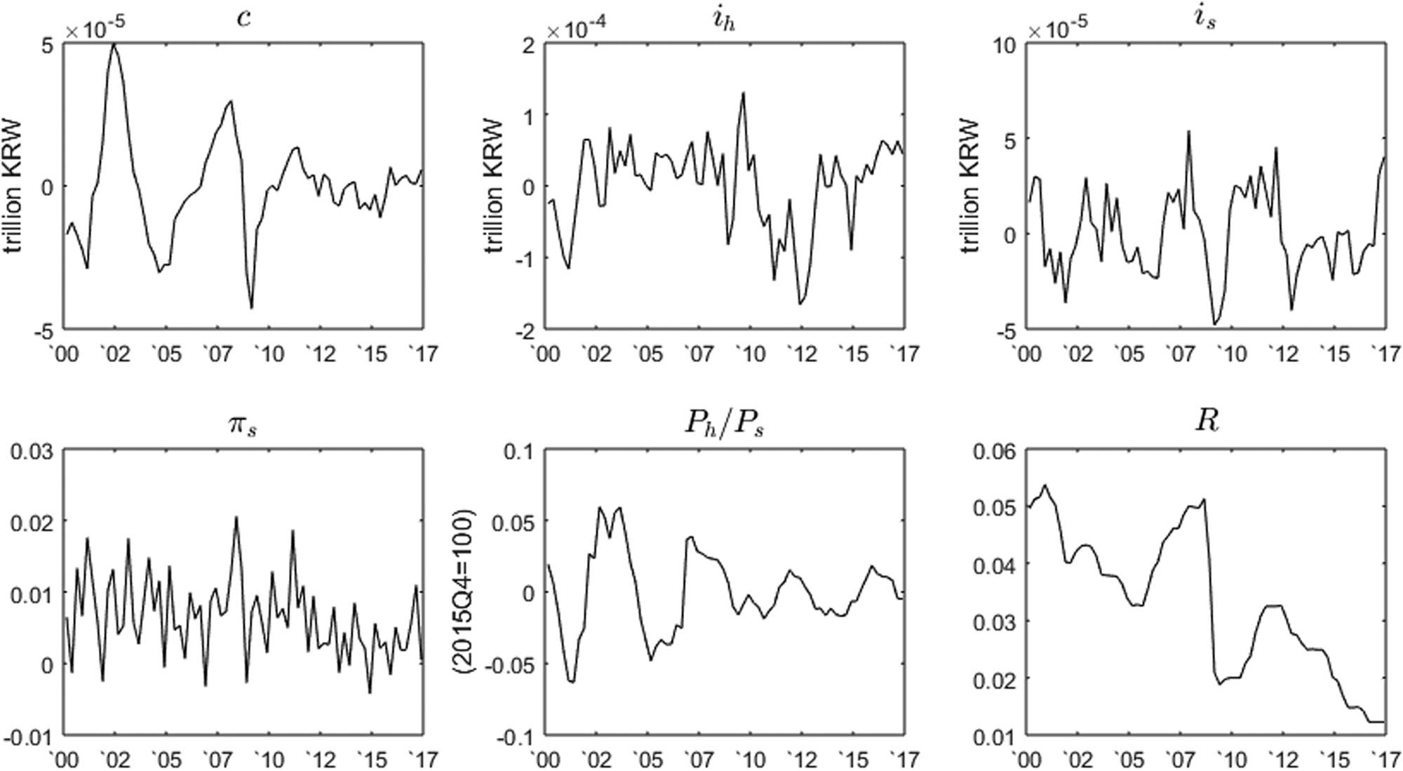
Hodrick–Prescott filtered sample data.
The model parameters are estimated using the Bayesian method, and the priors and the posteriors are presented in Table 1. The prior distributions for the parameters are determined by referring to Iacoviello and Neri (2010) and Lee and Song (2015). Following the convention in much of the literature, the prior distributions are set as loosely as possible to achieve reasonably good statistical properties for the whole estimation. We set the prior mean of
Priors and posteriors
| Parameters | Priors | Posteriors | ||||||
|---|---|---|---|---|---|---|---|---|
| Type | Mean | Std. | 5% | Mean | Mode | 95% | ||
| Habit formation |
|
Beta | 0.5 | 0.1 | 0.396 | 0.488 | 0.489 | 0.578 |
| Standard sector price stickiness |
|
Beta | 0.667 | 0.1 | 0.486 | 0.572 | 0.557 | 0.643 |
| Wage stickiness |
|
Beta | 0.667 | 0.1 | 0.580 | 0.657 | 0.654 | 0.733 |
| Standard household labor weight |
|
Beta | 0.65 | 0.05 | 0.555 | 0.633 | 0.635 | 0.711 |
| AR aggregate tech shock |
|
Beta | 0.6 | 0.1 | 0.519 | 0.646 | 0.675 | 0.773 |
| AR construction sector tech shock |
|
Beta | 0.6 | 0.1 | 0.506 | 0.620 | 0.627 | 0.732 |
| AR investment efficiency shock |
|
Beta | 0.6 | 0.1 | 0.456 | 0.555 | 0.559 | 0.656 |
| AR consumer preference shock |
|
Beta | 0.6 | 0.1 | 0.451 | 0.551 | 0.557 | 0.651 |
| AR housing demand shock |
|
Beta | 0.6 | 0.1 | 0.700 | 0.761 | 0.766 | 0.824 |
| MP interest rate smoothing |
|
Beta | 0.6 | 0.1 | 0.679 | 0.732 | 0.734 | 0.787 |
| Standard sector capital adjust. |
|
Inv. G | 45 | 2 | 35.209 | 48.781 | 45.421 | 62.440 |
| Housing sector capital adjust. |
|
Inv. G | 45 | 2 | 28.747 | 45.059 | 43.148 | 60.935 |
| Aggregate tech shock std. |
|
Inv. G | 0.001 | 0.05 | 0.0078 | 0.0116 | 0.0104 | 0.0150 |
| Housing sector tech shock std. |
|
Inv. G | 0.001 | 0.05 | 0.0132 | 0.0155 | 0.0151 | 0.0176 |
| Investment efficiency shock std. |
|
Inv. G | 0.001 | 0.05 | 0.019 | 0.026 | 0.024 | 0.033 |
| Consumer preference shock std. |
|
Inv. G | 0.001 | 0.05 | 0.016 | 0.020 | 0.020 | 0.025 |
| Housing demand shock std. |
|
Inv. G | 0.001 | 0.05 | 0.150 | 0.215 | 0.203 | 0.277 |
| MP shock std. |
|
Inv. G | 0.001 | 0.05 | 0.004 | 0.005 | 0.005 | 0.006 |
| MP inflation response |
|
Normal | 3 | 0.1 | 2.829 | 2.974 | 2.971 | 3.156 |
| MP output gap response |
|
Normal | 0 | 0.1 | 0.470 | 0.665 | 0.640 | 0.833 |
Note: The posteriors are estimated using the Bayesian method with 110,000 simulations. The first 10,000 simulations are considered a burn-in period and are discarded.
Abbreviations: AR – autoregressive; MP – monetary policy.
To check the model’s fit to the data, we compare the simulated moments from the model with those in the data and present the results in Table 2. The volatilities and correlations of most of the observable data are fairly well-matched with the model except for non-housing investments and the non-housing sector inflation rate.
Comparison of moments
|
|
|
|
|
|
|
|
|---|---|---|---|---|---|---|
| SD (%) | ||||||
| Data | 1.75 | 2.19 | 6.09 | 0.50 | 2.71 | 0.60 |
| Model | 1.48 | 2.18 | 5.80 | 0.53 | 2.30 | 0.48 |
|
Cross-correlation with
|
||||||
| Data | 0.16 | −0.04 | 1.00 | −0.01 | 0.19 | −0.21 |
| Model | 0.37 | 0.25 | 0.91 | −0.22 | 1.00 | −0.48 |
| Autocorrelation (order = 1) | ||||||
| Data | 0.84 | 0.57 | 0.64 | −0.15 | 0.84 | 0.86 |
| Model | 0.72 | 0.47 | 0.51 | 0.24 | 0.59 | 0.56 |
Note: Model moments are calculated using 10,000 simulations of the same length as the data. These simulations are generated by resampling the shocks identified over the sample period using the posterior means of the model parameters.
Figure 4 decomposes the historical housing production and real housing price data by the types of shocks identified over the sample period. We find that the soaring housing prices between 2006 and 2008 were mainly caused by the growing demand for houses. This excess demand for houses has faded since 2009. The sudden fall in technology shocks in residential construction explains the slowdown in housing production after 2011. The upswing in housing production since 2015 can be explained by the rebound in these technology shocks as well as the recovered demand for houses.
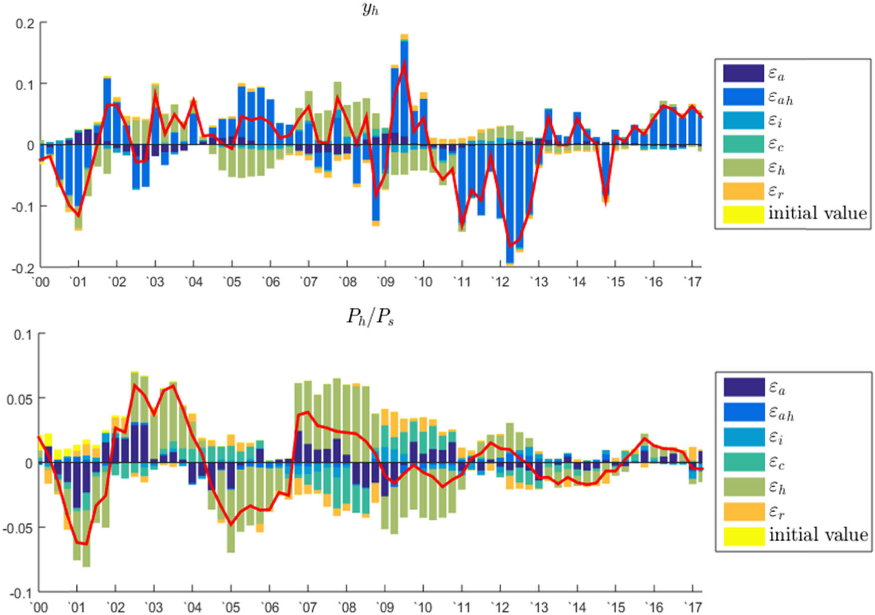
Historical decompositions.
3.3 Empirical analysis
This subsection provides the response functions of the endogenous variables to each shock and checks whether the model’s predictions are consistent with the stylized facts given by theory and data. Figure 5 shows the responses of real GDP (
Responses to a productivity shock in the non-housing production sector (
Figure 6 shows the responses to a productivity shock (
Responses to a productivity shock in the housing production sector (
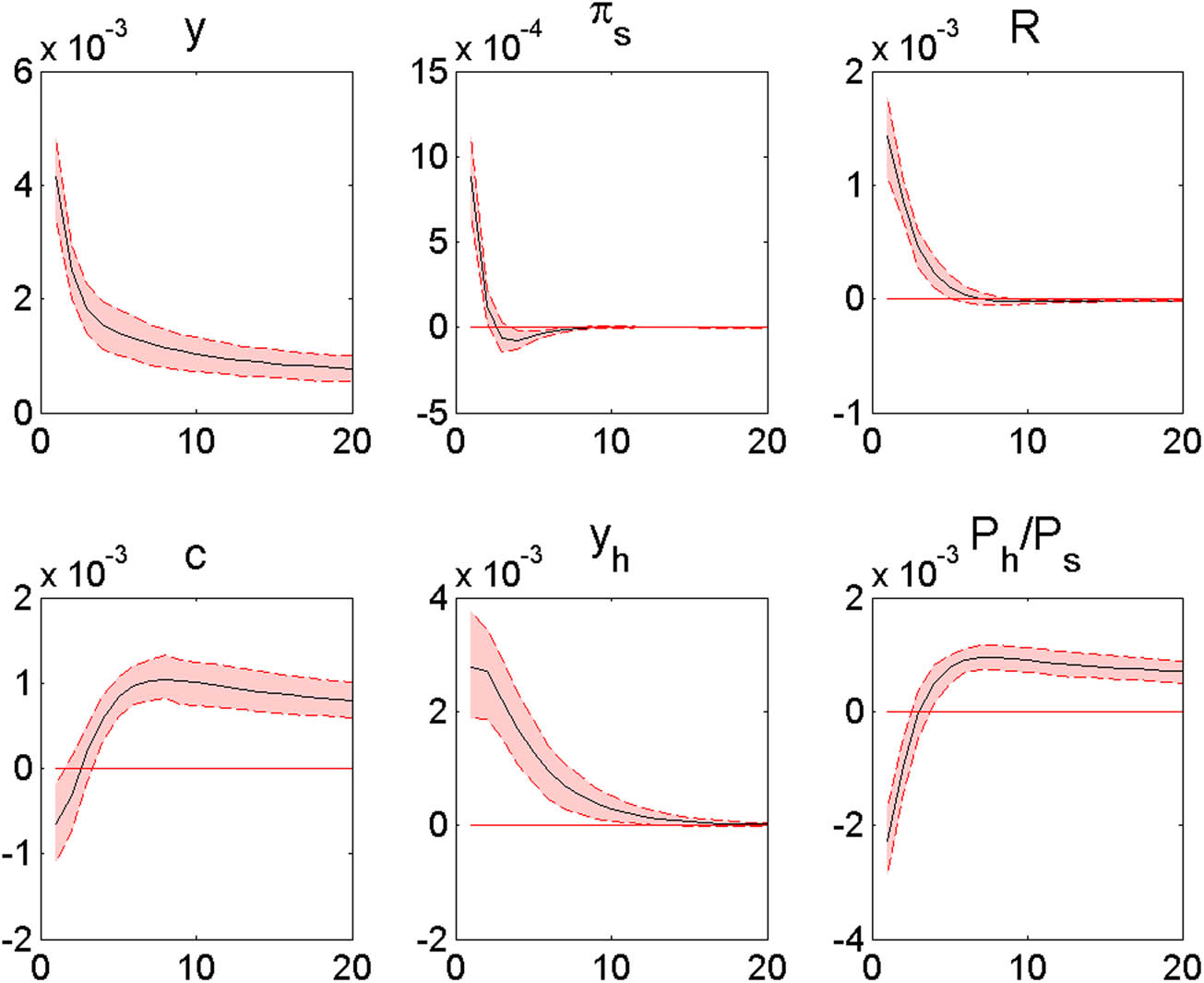
Figure 7 shows the responses to a consumption preference shock (
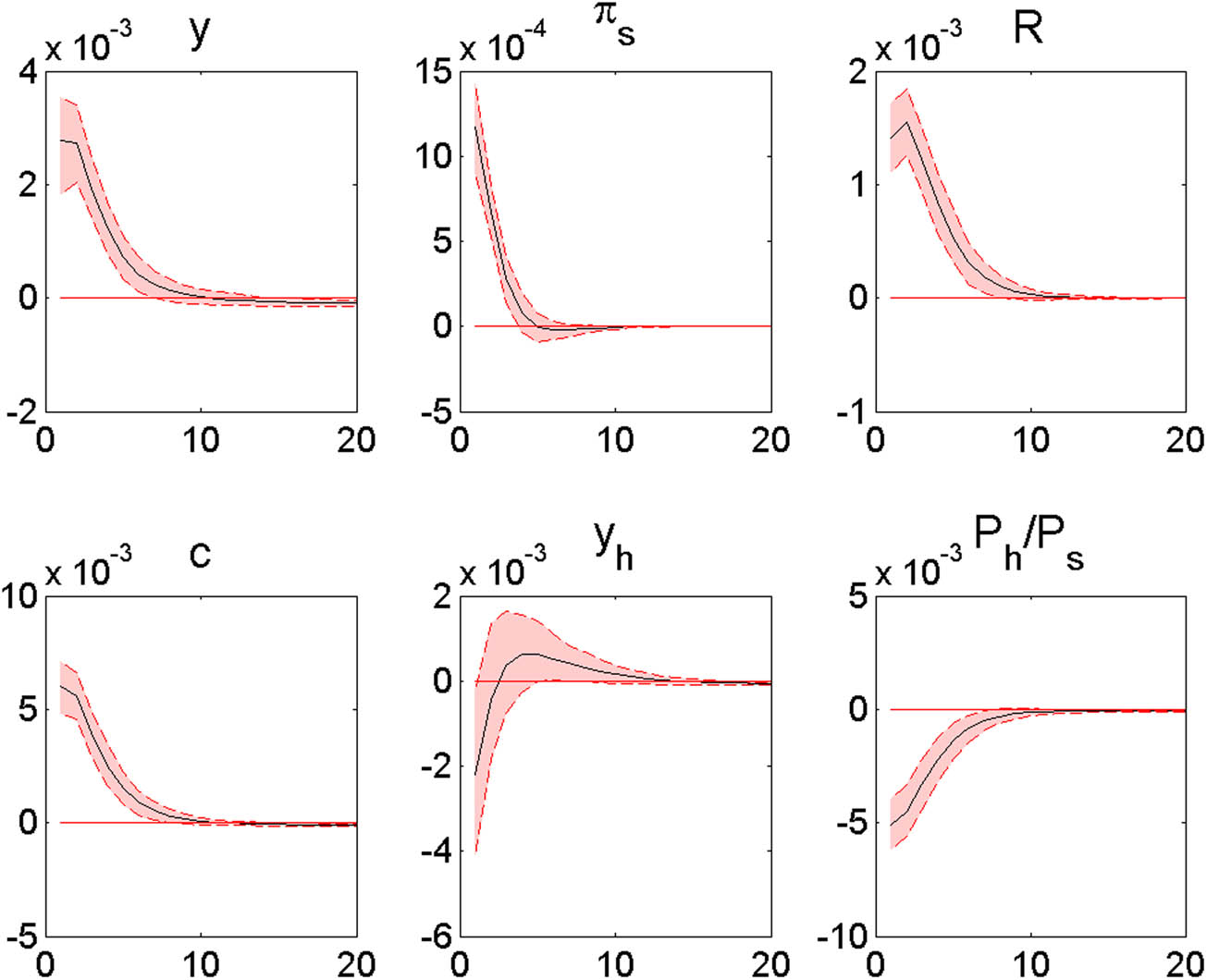
Responses to a consumption preference shock (
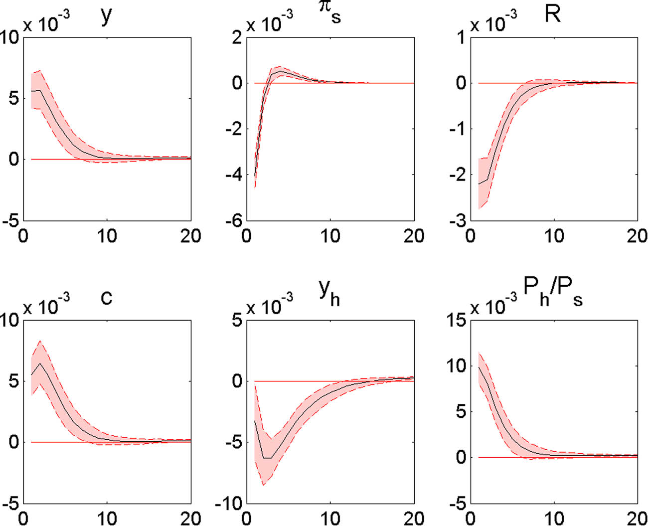
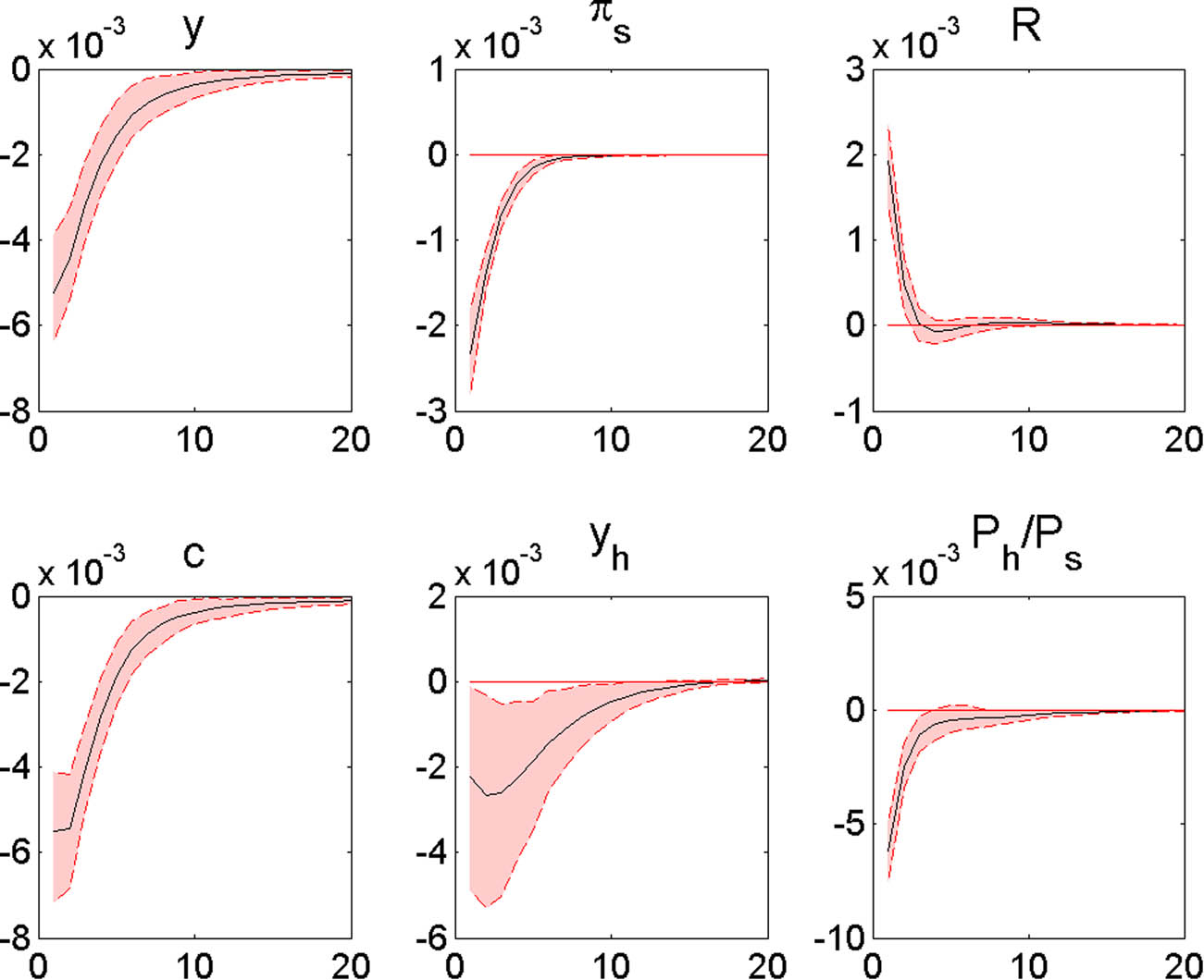
Figure 8 shows the responses to a negative housing preference shock (
Responses to a negative housing preference shock (
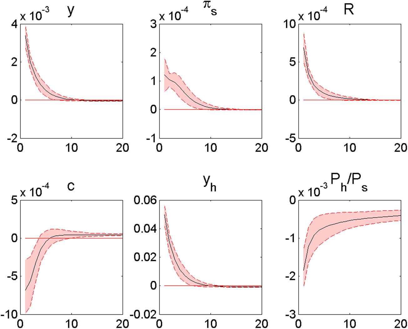
Figure 9 shows the responses to an investment efficiency shock (
Responses to an investment efficiency shock (
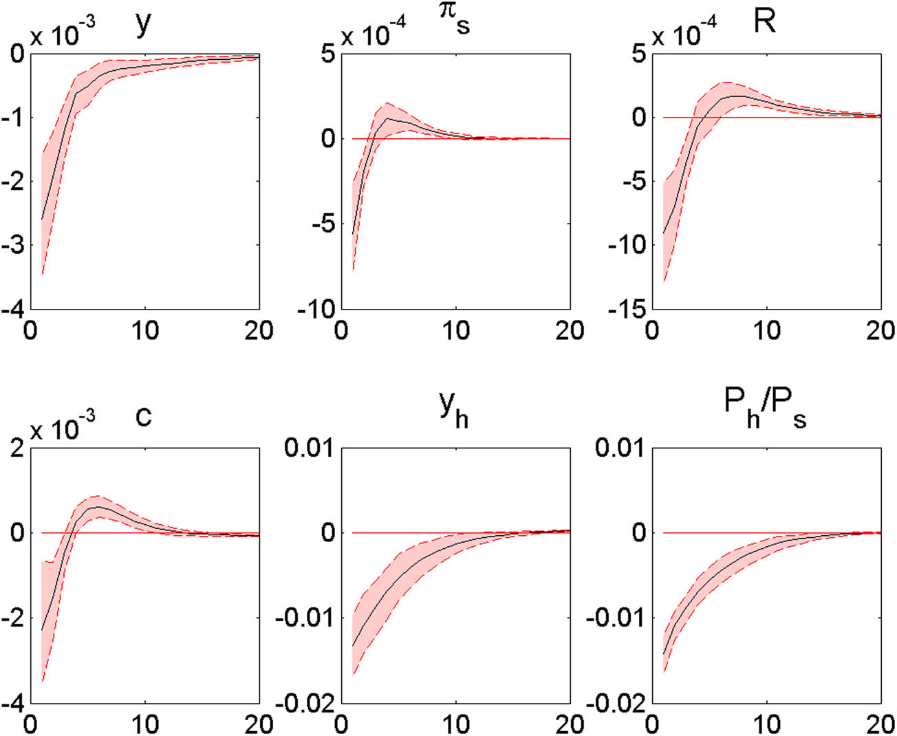
Figure 10 shows the responses to an exogenous MP shock (
Responses to an MP shock
Table 3 shows the forecasting error variance decomposition results for key macroeconomic variables. The table shows that consumption (
Forecasting error variance decomposition of structural shocks
|
|
|
|
|||||||
|---|---|---|---|---|---|---|---|---|---|
| Quarter | 1 | 4 | 20 | 1 | 4 | 20 | 1 | 4 | 20 |
|
|
0.320 | 0.408 | 0.386 | 0.694 | 0.631 | 0.634 | 0.368 | 0.460 | 0.458 |
|
|
0.115 | 0.076 | 0.069 | 0.001 | 0.001 | 0.002 | 0.034 | 0.023 | 0.023 |
|
|
0.081 | 0.091 | 0.085 | 0.057 | 0.068 | 0.067 | 0.146 | 0.233 | 0.239 |
|
|
0.060 | 0.049 | 0.047 | 0.011 | 0.012 | 0.012 | 0.051 | 0.045 | 0.049 |
|
|
0.169 | 0.123 | 0.169 | 0.031 | 0.028 | 0.027 | 0.140 | 0.103 | 0.100 |
|
|
0.255 | 0.252 | 0.244 | 0.206 | 0.261 | 0.258 | 0.260 | 0.136 | 0.132 |
|
|
|
|
|||||||
|---|---|---|---|---|---|---|---|---|---|
| Quarter | 1 | 4 | 20 | 1 | 4 | 20 | 1 | 4 | 20 |
|
|
0.313 | 0.410 | 0.400 | 0.005 | 0.032 | 0.041 | 0.273 | 0.277 | 0.251 |
|
|
0.004 | 0.003 | 0.002 | 0.924 | 0.865 | 0.845 | 0.009 | 0.008 | 0.011 |
|
|
0.366 | 0.300 | 0.278 | 0.001 | 0.001 | 0.001 | 0.071 | 0.081 | 0.074 |
|
|
0.042 | 0.022 | 0.023 | 0.064 | 0.091 | 0.101 | 0.535 | 0.569 | 0.592 |
|
|
0.004 | 0.003 | 0.041 | 0.003 | 0.005 | 0.006 | 0.014 | 0.008 | 0.019 |
|
|
0.270 | 0.263 | 0.255 | 0.002 | 0.005 | 0.007 | 0.099 | 0.058 | 0.052 |
|
|
|
|
|||||||
|---|---|---|---|---|---|---|---|---|---|
| Quarter | 1 | 4 | 20 | 1 | 4 | 20 | 1 | 4 | 20 |
|
|
0.146 | 0.195 | 0.188 | 0.408 | 0.510 | 0.484 | 0.101 | 0.065 | 0.058 |
|
|
0.002 | 0.002 | 0.001 | 0.000 | 0.000 | 0.000 | 0.012 | 0.018 | 0.042 |
|
|
0.037 | 0.054 | 0.054 | 0.103 | 0.100 | 0.092 | 0.045 | 0.031 | 0.025 |
|
|
0.002 | 0.002 | 0.007 | 0.031 | 0.021 | 0.019 | 0.821 | 0.842 | 0.753 |
|
|
0.761 | 0.709 | 0.712 | 0.179 | 0.118 | 0.165 | 0.017 | 0.039 | 0.117 |
|
|
0.053 | 0.039 | 0.038 | 0.280 | 0.250 | 0.239 | 0.004 | 0.005 | 0.006 |
Note: The variance decomposition indicates the amount of information that each structural shock contributes to the endogenous macroeconomic variables. This decomposition shows how much of the forecasting error variance of each macroeconomic variable can be explained by each of the five structural shocks. The forecasting error variances of the endogenous variables explained by each structural shock in a given period sum to one.
4 Comparative static analyses
4.1 Lowering the LTV ceiling
To examine the macroeconomic effects of household debt deleveraging, we reduce the LTV ceiling from the baseline fixed at 70% in the estimation to 50%. As the LTV ratio declines, borrowers face relatively high pressure to deleverage. In the case of housing preferences and MP shocks, the impact of the LTV ratio is more pronounced.
Figure 11 shows that a negative housing preference shock decreases the relative price of housing in the short term when the LTV ceiling is reduced below the baseline. However, the relative price of housing is higher than the baseline prediction as time passes. In contrast, the macroeconomic indicators, such as consumption and non-housing and housing production, contract less when the LTV ceiling is reduced relative to the baseline following a negative housing preference shock. As households already borrow less under a 50% LTV ceiling and the marginal utility from housing services is even higher relative to the baseline, a negative housing preference shock is less likely to change the marginal rate of substitution between housing and non-housing consumption. Non-housing consumption increases following a negative housing preference shock, meaning that prices and, thus, nominal interest rates rise according to the MP rule as well. As a result, a downward adjustment of the LTV ratio significantly insulates the real economy from the impact of a negative housing preference shock relative to the baseline outcomes.
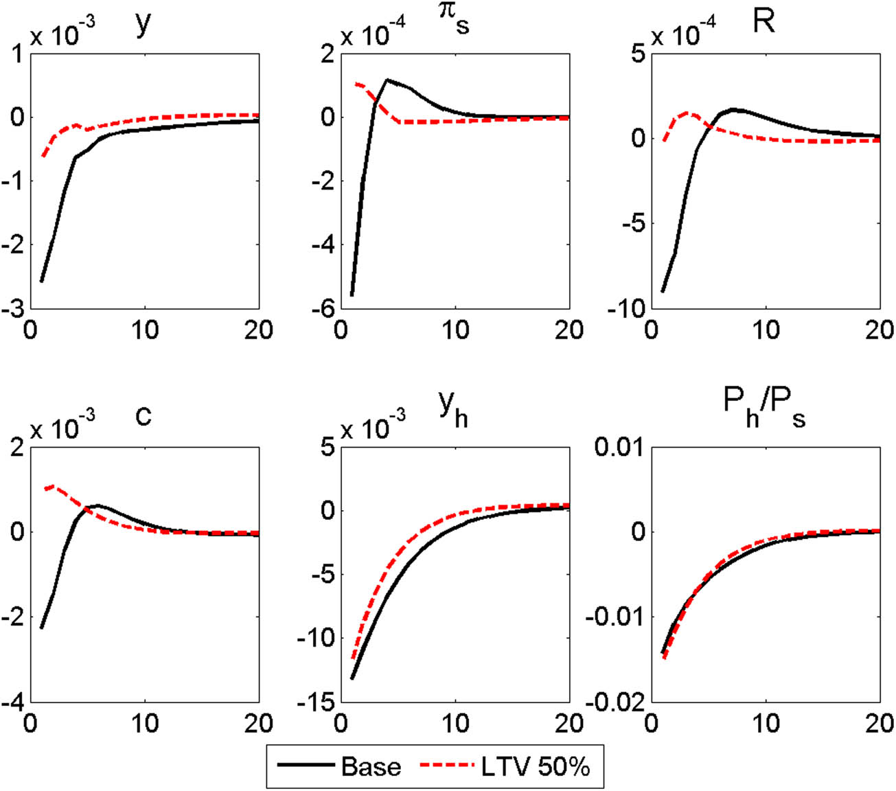
Responses to a negative housing preference shock (
When the LTV ceiling is adjusted downward, the effects of exogenous monetary shocks on real GDP, inflation, consumption, and housing production are also relatively moderate compared to the baseline estimates, as shown in Figure 12. However, the relative housing price declines more than in the baseline case because housing prices respond more elastically to the interest rate than the general prices. As in the case of a negative housing preference shock, the downward adjustment of the LTV ceiling attenuates the impacts of an exogenous monetary shock and limits the effects of economic fluctuations.
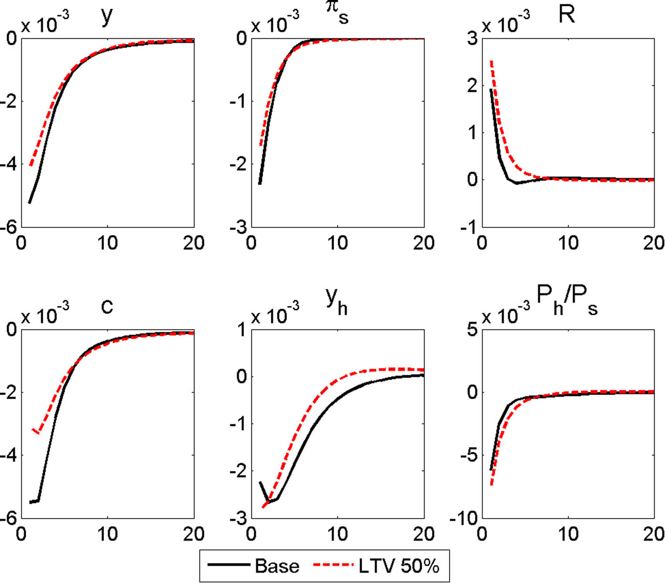
Responses to an MP shock (
4.2 Housing-price-augmented MP rule
We now modify Taylor’s rule to reflect housing prices as follows:
Here,
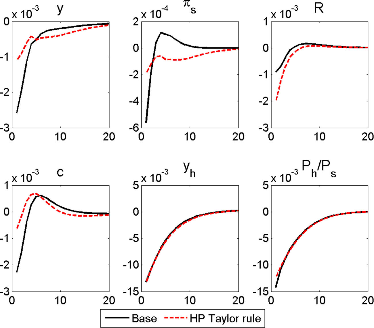
Responses to a negative housing preference shock
In the case of an exogenous MP shock, a higher interest rate lowers real GDP, consumption, residential construction investment, and housing and non-housing prices, as presented in Figure 14. A rise in nominal interest rates causes non-housing prices to decline as a result of reduced consumption and housing prices as borrowers face tighter collateral constraints and lower demand for houses. The nominal interest rate then decreases as the consumer price and asset prices fall over time. When we compare these results to the corresponding results in the baseline cases, the differences are very negligible. Thus, the monetary response to housing price inflation has limited macroeconomic implications in Korea.
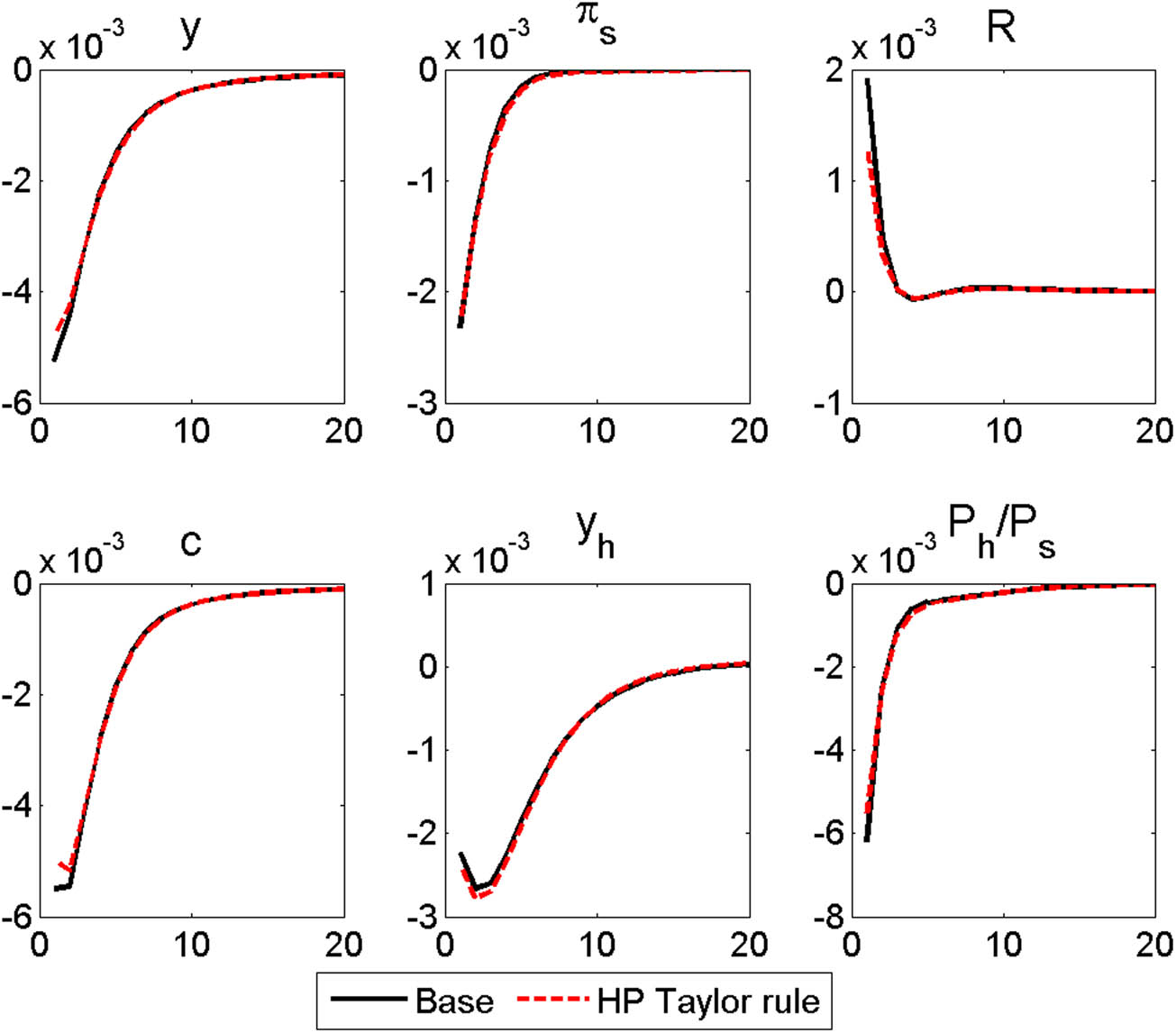
Responses to an MP shock
4.3 Lowering the LTV ceiling and setting a house-price-augmented MP rule
Now, we consider the hypothetical situation in which the LTV ceiling is reduced to 50% and the central bank follows a new MP rule that takes housing prices into account. In this case, the changes in real GDP, consumption, and inflation in response to a negative housing preference shock, considering the baseline, decrease only slightly or even increase, as presented in Figure 15. Owing to the downward adjustment of the LTV ratio, which regulates the maximum percent of the value of a purchased house that a household can borrow, the impact of a negative housing preference shock is limited. The decline in housing prices reinforces this mitigating effect by adjusting the nominal interest rate down to better absorb the shock relative to the baseline case.
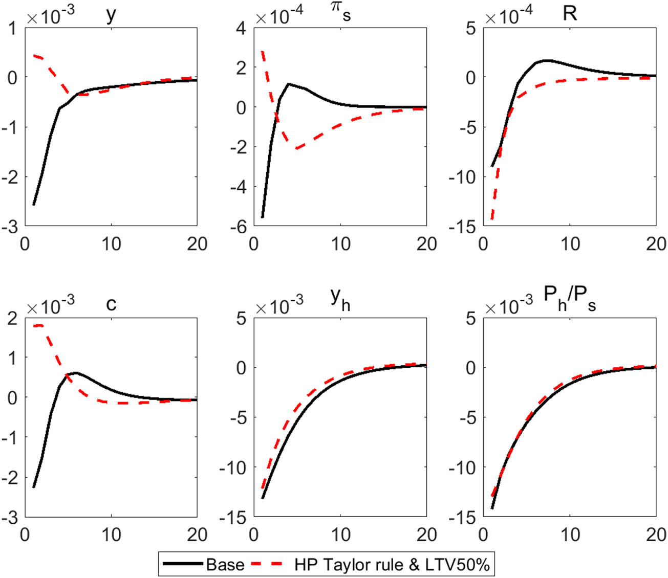
Response to a negative housing preference shock (
Figure 16 shows the responses to an MP shock in the baseline case and the hypothetical scenario. Because an MP shock has little impact on economic fluctuations, most of the fluctuations must be attributed to the downward adjustment of the LTV ceiling. As the nominal interest rate rises, real GDP, consumption, and inflation decline. However, they fall more gradually in the hypothetical scenario than in the baseline case. This result can be attributed to the decrease in the burden of interest payments. As the stronger LTV restriction limits the amount that borrowers can afford to borrow at the margin, the change in borrowers’ interest payments due to the rise in the interest rate is less severe than in the baseline. Housing prices, which are most sensitive to nominal interest rates, decline rapidly, and their decline, relative to non-housing prices, is greater than in the baseline case. The lower the LTV ceiling is, the harder it becomes to borrow funds using a house as collateral, and, hence, housing prices become more sensitive to changes in interest rates.
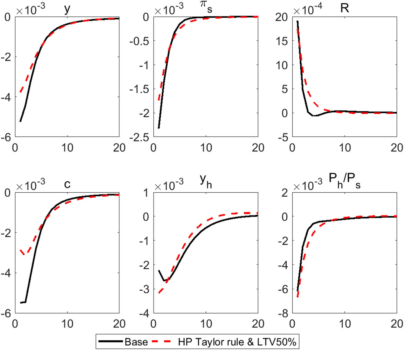
Response to an MP shock (
These results suggest that the economy can be further insulated from the impacts of a negative housing preference shock by introducing a tighter LTV ceiling and an MP rule that considers housing price inflation.
4.4 Welfare distribution after shocks
A welfare analysis can reveal the distinct responses of the borrowers and savers, separately, to a given shock (Menno & Oliviero, 2020). In this subsection, we decompose the welfare response to each shock by household type and observe the changes in this response when the LTV requirement tightens. Figure 17 presents the welfare responses under an LTV ratio of 70%. When the economy is hit by a consumption preference or housing sector productivity shock, the borrowers’ welfare increases relative to that of the savers. As the borrowers’ value of housing increases under these shocks, they accumulate more housing for current use and as collateral for future consumption, resulting in greater welfare for the borrowers.
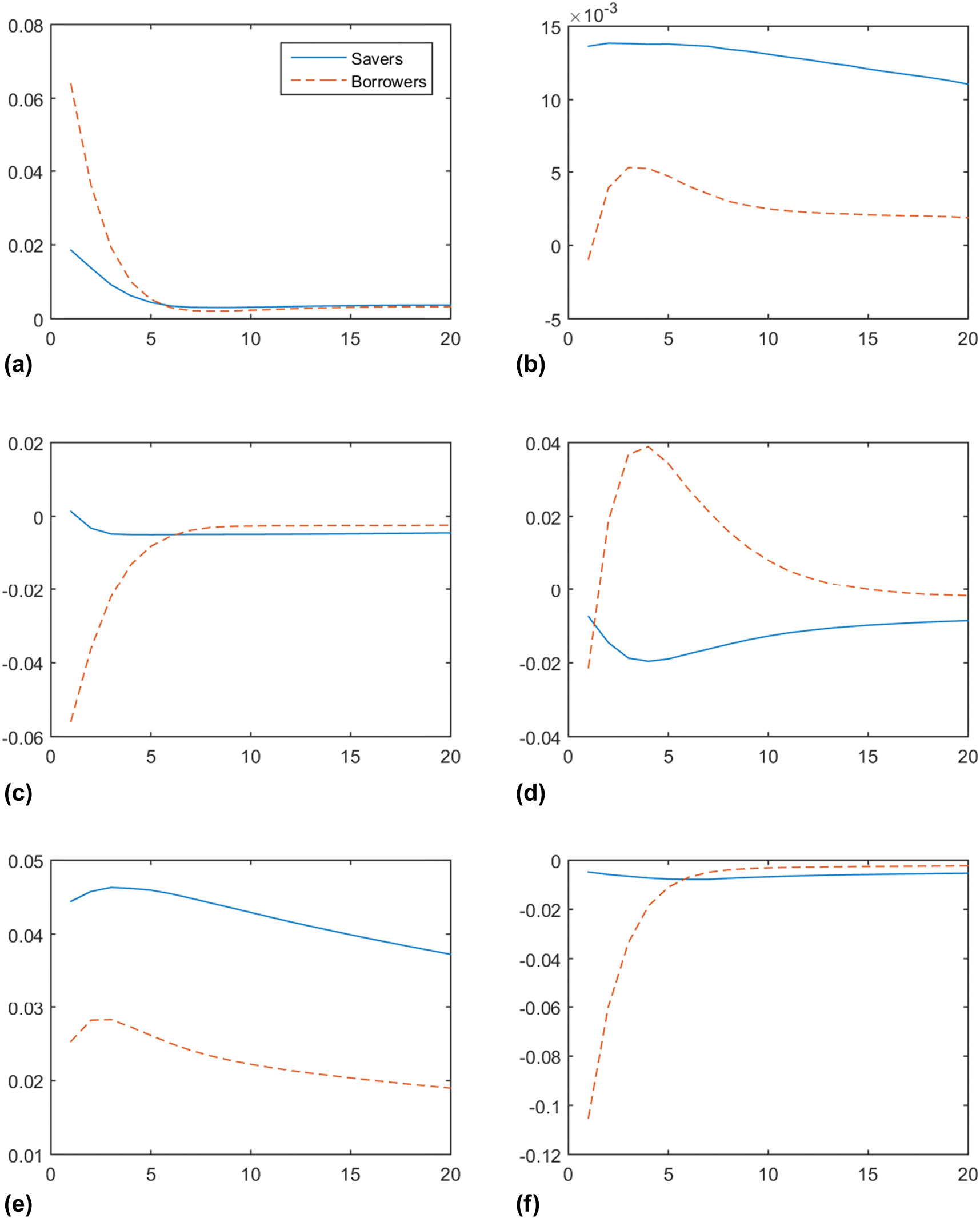
Welfare responses by type of shock with a 70% LTV ceiling: savers vs borrowers. (a) Consumption preference shock (
Figure 18 presents the welfare responses when the LTV requirement is reduced to 50%. Under this tighter collateral requirement, the scale of the y-axis alone shows that the welfare variations are relatively subdued compared to the case with a looser collateral constraint. Interestingly, the welfare responses to the consumption preference and housing sector productivity shocks are reversed. In the previous case, these shocks lead to greater welfare for the borrowers than for the savers. With a lower LTV requirement, however, this result no longer occurs, although the differences are not large. One possible explanation for this reversal is that a tighter LTV requirement reduces the collateral value of housing and, thus, the borrowers’ ability to substitute consumption intertemporally is limited. This explanation is only partial, and further analysis is required to fully understand this result. We leave this for future research. For now, we show that deleveraging through a tighter LTV requirement has a distributional welfare effect, which many other studies have overlooked (Cloyne, Ferreira, & Surico, 2020; Justiniano et al., 2015, 2019; Liu and Ou, 2021).
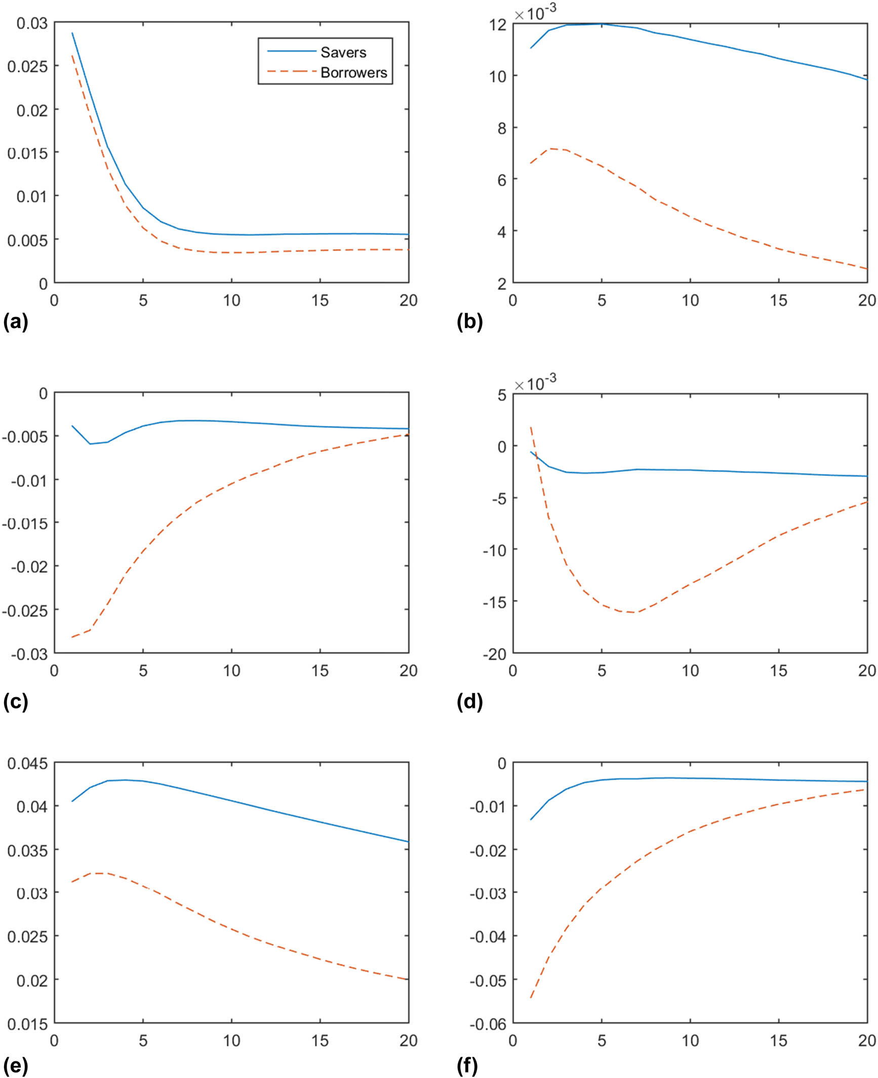
Welfare responses by type of shock with a 50% LTV ceiling: savers vs borrowers. (a) Consumption preference shock (
4.5 Sensitivity of the MP rule to housing price shocks
In the previous analysis, we set the value of
To conduct robustness checks on the value of
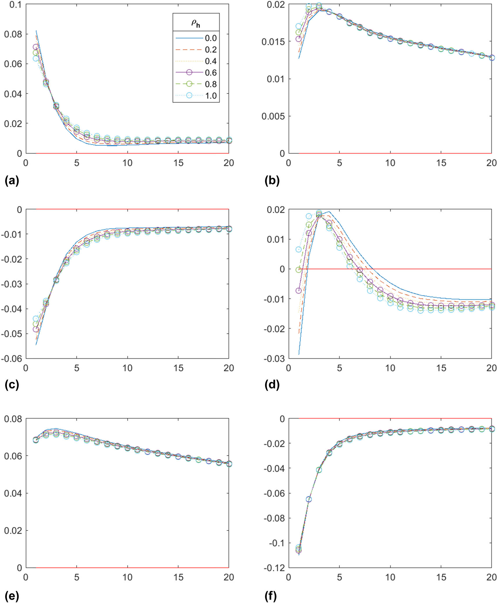
Aggregate welfare (
In the case of other shocks, a policy rule that incorporates housing prices serves to increase aggregate welfare. In particular, this policy rule works fairly well when the economy is hit by a demand shock rather than a supply shock. In the case of a preference shock, regardless of whether it is housing-related, aggregate welfare increases when the central bank reacts procyclically in response to the shock. However, if the economy is hit by a supply shock, a proactive MP in response to a housing price hike leads to lower aggregate welfare than in the baseline case. These results reveal that MP should respond asymmetrically depending on the source of a shock to facilitate overall economic welfare. As Cloyne et al., (2020) point out, these results can be interpreted as the impact of an interest rate shock decreasing as the proportion of mortgage payments decreases.
5 Conclusion and policy implications
This study systematically discusses the effects of the MP in Korea during household debt deleveraging, which is not widely studied in developing countries and emerging economies. Although the household debt associated with housing is an essential factor in MP operation, high interest rates and underdeveloped consumer financial markets make policymakers overlook its significance. With the development of consumer financial markets and the expansion of housing demand since the early 2000s, Korea’s household debt began to skyrocket and reached a doorstep to concern and manage its size and growth. This provides an essential motivation for this study. To the best of our knowledge, only a few studies examine how effective an MP rule adjusted for housing prices would be to various structural shocks under the LTV restrictions. Our empirical results are meaningful in that the housing-price-adjusted MP rule is found to effectively stabilize the economy in response to a demand shock, which is not addressed in previous studies (Iacoviello & Neri, 2010).
Household debt has reached a record high and is considered one of the most serious problems faced by the Korean economy. Both the level and the growth rate of debt are unprecedented, and the debt is highly concentrated in the housing market. Hence, concerns are growing that underperformance in the housing market will trigger deleveraging, which may debilitate the housing market and, eventually, the overall financial system. These concerns should be assessed quantitatively to gauge their potential risk and determine the relevant policy measures.
This study constructs and estimates a DSGE model based on Korean data. Our model incorporates heterogeneous households with different subjective discount rates, collateral constraints, and a housing production sector. Based on this model, we conduct comparative static analyses using various external shocks and analyze the effects of these shocks on output, consumption, general prices, housing production, interest rates, and housing prices relative to the baseline. In particular, we investigate a hypothetical scenario in which the LTV ceiling is set below its current level and the interest rate responds to housing price fluctuations in an otherwise standard MP rule.
The simulation results show that tighter LTV restrictions can reduce the influence of external shocks on the economy. As a lower LTV ceiling reduces the amount of debt that borrower households can afford, the deleveraging effect, which is mostly caused by borrowers’ re-optimization, is alleviated relative to the baseline case. When the MP rule is adjusted to include housing prices in its reaction function, MP becomes more sensitive to housing price movements and tends to allow the housing market and the macroeconomy to stabilize more quickly than in the baseline case. For example, a negative housing preference shock lowers the interest rate directly to stabilize housing prices. As a result, the decrease in consumption and real GDP is smaller than in the baseline case, in which interest rates are adjusted indirectly through inflation and the output gap following a shock.
When the MP rule that incorporates the housing price gap is introduced in combination with a tighter LTV ceiling to mitigate the impact of deleveraging, any negative shocks to housing prices are countered by both lower interest rates and the decumulation of debts. The responses of real GDP, consumption, and investment to negative housing price shocks are more subdued compared to the cases in which policy adjustments to the housing price gap are not made.
Finally, we investigate the optimal MP rule with respect to
Tightening LTV regulations restricts home buyers’ lending limits, thereby restraining demand and either mitigating housing price rises or inducing price declines. However, tighter regulations can deprive households of homeownership if they lack sufficient cash. Thus, although tightening LTV regulations can improve macroeconomic resiliency, different LTV ceilings for socially disadvantaged households and credit from public institutions should be provided in parallel.
Based on our analyses and findings, we suggest some future research topics. First, it would be interesting to include the dynamic processes by which macroeconomic variables fluctuate when the LTV ceiling changes from 70% to 50%. Doing so would require developing an entirely different set of dynamic models to track the transitions of macroeconomic variables over time. Second, a further investigation on the benefits/costs of LTV ceilings can reveal which households (i.e., borrowers or savers) would benefit from the restriction, potentially suggesting meaningful intuitions about the political economy feasibility of an LTV ceiling.
Acknowledgment
The authors appreciate helpful comments and suggestions from Kai Carstensen (the editor), Hyeongjun Kim, Sungtaek Yim, Jinyoung Yu, Daehyeon Park, Daehan Kim, and two anonymous referees. This study is the extended version of the earlier research project titled Analysis on Household Debt Deleveraging under Heterogeneous Preferences. Song, acknowledges the support from the Bank of Korea for the project and the research grant from Hankuk University of Foreign Studies. Ryu acknowledges the support by the Ministry of Education of the Republic of Korea and the National Research Foundation of Korea (NRF-2020S1A5A2A01045882). The views and conclusions of this study are those of the authors and do not necessarily reflect those of the Bank of Korea.
-
Conflict of interest: Authors state no conflict of interest.
References
Arcand, J. L., Berkes, E., & Panizza, U. (2015). Too much finance? Journal of Economic Growth, 20(2), 105–148. 10.1007/s10887-015-9115-2.Suche in Google Scholar
Benigno, P., Eggertsson, G. B., & Romei, F. (2020). Dynamic debt deleveraging and optimal monetary policy. American Economic Journal: Macroeconomics, 12(2), 310–350. 10.1257/mac.20160124.Suche in Google Scholar
Cecchetti, S. G., & Kharroubi, E. (2012). Reassessing the impact of finance on growth. BIS Working Paper, 381. Available at SSRN: https://ssrn.com/abstract=2117753Suche in Google Scholar
Cecchetti, S. G., Mohanty, M. S., & Zampolli, F. (2011). The real effects of debt. BIS Working Paper, 352. Available at SSRN: https://ssrn.com/abstract=1946170Suche in Google Scholar
Cerutti, E., & Claessens, S. (2017). The great cross-border bank deleveraging: Supply constraints and intra-group frictions. Review of Finance, 21(1), 201–236. 10.1093/rof/rfw002.Suche in Google Scholar
Chun, D., Cho, H., & Ryu, D. (2020). Economic indicators and stock market volatility in an emerging economy. Economic Systems, 44(2), 100788. 10.1016/j.ecosys.2020.100788.Suche in Google Scholar
Chung, C. Y., Cho, S. J., Ryu, D., & Ryu, D. (2019). Institutional blockholders and corporate social responsibility. Asian Business & Management, 18(3), 143–186. 10.1057/s41291-018-00056-w.Suche in Google Scholar
Cloyne, J., Ferreira, C., & Surico, P. (2020). Monetary policy when households have debt: New evidence on the transmission mechanism. Review of Economic Studies, 87(1), 102–129. 10.1093/restud/rdy074.Suche in Google Scholar
Davis, M. A., & Heathcote, J. (2005). Housing and the business cycle. International Economic Review, 46(3), 751–784. 10.1111/j.1468-2354.2005.00345.x.Suche in Google Scholar
Di Maggio, M., Kermani, A., Keys, B. J., Piskorski, T., Ramcharan, R., Seru, A., & Yao, V. (2017). Interest rate pass-through: Mortgage rates, household consumption, and voluntary deleveraging. American Economic Review, 107(11), 3550–3588. 10.1257/aer.20141313.Suche in Google Scholar
Dynan, K. E. (2000). Habit formation in consumer preferences: Evidence from panel data. American Economic Review, 90(3), 391–406. 10.1257/aer.90.3.391.Suche in Google Scholar
Gerali, A., Neri, S., Sessa, L., & Signoretti, F. M. (2010). Credit and banking in a DSGE model of the Euro area. Journal of Money, Credit and Banking, 42(s1), 107–141. 10.1111/j.1538-4616.2010.00331.x.Suche in Google Scholar
Guerrieri, L., & Iacoviello. M. (2017). Collateral constraints and macroeconomic asymmetries. Journal of Monetary Economics, 90, 28–49. 10.1016/j.jmoneco.2017.06.004.Suche in Google Scholar
Iacoviello, M. (2005). House prices, borrowing constraints, and monetary policy in the business cycle. American Economic Review, 95(3), 739–764. 10.1257/0002828054201477.Suche in Google Scholar
Iacoviello, M., & Neri, S. (2010). Housing market spillovers: Evidence from an estimated DSGE model. American Economic Journal: Macroeconomics, 2(2), 125–164. 10.1257/mac.2.2.125.Suche in Google Scholar
Jang, H., Song, Y., & Ahn, K. (2020). Can government stabilize the housing market? The evidence from South Korea. Physica A: Statistical Mechanics and its Applications, 550, 124114. 10.1016/j.physa.2019.124114.Suche in Google Scholar
Justiniano, A., Primiceri, G. E., & Tambalotti, A. (2015). Household leveraging and deleveraging. Review of Economic Dynamics, 18(1), 3–20. 10.1016/j.red.2014.10.003.Suche in Google Scholar
Justiniano, A., Primiceri, G. E., & Tambalotti, A. (2019). Credit supply and the housing boom. Journal of Political Economy, 127(3), 1317–1350. Retrieved from https://www.journals.uchicago.edu/doi/pdf/10.1086/70144010.3386/w20874Suche in Google Scholar
Kim, H. M. (2017). Ethnic connections, foreign housing investment and locality: A case study of Seoul. International Journal of Housing Policy, 17(1), 120–144. 10.1080/14616718.2016.1189683.Suche in Google Scholar
Kim, H., Batten, J. A., & Ryu, D. (2020). Financial crisis, bank diversification, and financial stability: OECD countries. International Review of Economics and Finance. 65, 94–104. 10.1016/j.iref.2019.08.009.Suche in Google Scholar
Kim, H., Cho, H., & Ryu, D. (2018a). An empirical study on credit card loan delinquency. Economic Systems, 42(3), 437–449. 10.1016/j.ecosys.2017.11.003.Suche in Google Scholar
Kim, H., Cho, H., & Ryu, D. (2018b). Characteristics of mortgage terminations: An analysis of a loan-level dataset. Journal of Real Estate Finance and Economics, 57(4), 647–676. 10.1007/s11146-017-9620-5.Suche in Google Scholar
Kim, H., Cho, H., & Ryu, D. (2019). Default risk characteristics of construction surety bonds. Journal of Fixed Income, 29(1), 77–87. 10.3905/jfi.2019.29.1.077.Suche in Google Scholar
Koo, R. C. (2009). The holy grail of macroeconomics: Lessons from Japan’s great recession (revised edition), Singapore, Asia: John Wiley & Sons.Suche in Google Scholar
Law, S. H., & Singh, N. (2014). Does too much finance harm economic growth? Journal of Banking & Finance, 41, 36–44. 10.1016/j.jbankfin.2013.12.020.Suche in Google Scholar
Lee, J., & Ryu, D. (2019a). How does FX liquidity affect the relationship between foreign ownership and stock liquidity? Emerging Markets Review. 39, 101–119. 10.1016/j.ememar.2019.04.001.Suche in Google Scholar
Lee, J., & Ryu, D. (2019b). The impacts of public news announcements on intraday implied volatility dynamics. Journal of Futures Markets. 39(6), 656–685. 10.1002/fut.22002.Suche in Google Scholar
Lee, J., & Song, J. (2015). Housing and business cycles in Korea: A multi-sector Bayesian DSGE approach. Economic Modelling. 45, 99–108. 10.1016/j.econmod.2014.11.009.Suche in Google Scholar
Lindé, J. (2018). DSGE models: Still useful in policy analysis?. Oxford Review of Economic Policy. 34(1–2), 269–286. 10.1093/oxrep/grx058.Suche in Google Scholar
Liu, C., & Ou, Z. (2021). What determines China’s housing price dynamics? New evidence from a DSGE‐VAR. International Journal of Finance and Economics. Forthcoming. 10.1002/ijfe.1962.Suche in Google Scholar
McKinsey Global Institute. (2010). Debt and deleveraging: The global credit bubble and its economic consequences. McKinsey Report. Retrieved from https://www.mckinsey.com/∼/media/mckinsey/featured%20insights/employment%20and%20growth/debt%20and%20deleveraging/mgi_debt_and_deleveraging_executive_summary.ashxSuche in Google Scholar
Menno, D., & Oliviero, T. (2020). Financial intermediation, house prices, and the welfare effects of the US Great Recession. European Economic Review, 129, 103568. 10.1016/j.euroecorev.2020.103568.Suche in Google Scholar
Mian, A., Sufi, A., & Verner, E. (2017). Household debt and business cycles worldwide. Quarterly Journal of Economics, 132(4), 1755–1817. 10.1093/qje/qjx017.Suche in Google Scholar
Moon, B. (2018). Housing investment, default risk, and expectations: Focusing on the Chonsei market in Korea. Regional Science and Urban Economics, 71, 80–90. 10.1016/j.regsciurbeco.2018.05.004.Suche in Google Scholar
Noh, S. (2020). The effects and origins of house price uncertainty shocks. Working Paper, Korea Capital Market Institute. Available at https://ssrn.com/abstract=353035010.2139/ssrn.3530350Suche in Google Scholar
Ryu, D., Kim, M. H., & Ryu, D. (2019). The effect of international strategic alliances on firm performance before and after the global financial crisis. Emerging Markets Finance and Trade, 55(15), 3539–3552. 10.1080/1540496X.2019.1664466.Suche in Google Scholar
Ryu, D., Ryu, D., & Yang, H. (2020). Investor sentiment, market competition, and financial crisis: Evidence from the Korean stock market. Emerging Markets Finance and Trade, 56(8), 1804–1816. 10.1080/1540496X.2019.1675152.Suche in Google Scholar
Ryu, D., Webb, R. I., & Yu, J. (2020). Bank sensitivity to international regulatory reform: The case of Korea. Investment Analysts Journal. 49(2), 149–162. 10.1080/10293523.2020.1775989.Suche in Google Scholar
Ryu, D., & Yu, J. (2020). Hybrid bond issuances by insurance firms. Emerging Markets Review. 45, 100722. 10.1016/j.ememar.2020.100722.Suche in Google Scholar
Ryu, D., & Yu, J. (2021). Nonlinear effect of subordinated debt changes on bank performance. Finance Research Letters, 38, 101496. 10.1016/j.frl.2020.101496.Suche in Google Scholar
Seok, S. I., Cho, H., & Ryu, D. (2020). The information content of funds from operations and net income in real estate investment trusts. North American Journal of Economics and Finance. 51, 101063. 10.1016/j.najef.2019.101063.Suche in Google Scholar
Seppecher, P., & Salle, I. (2015). Deleveraging crises and deep recessions: A behavioural approach. Applied Economics, 47(34–35), 3771–3790. 10.1080/00036846.2015.1021456.Suche in Google Scholar
Shim, H., Chung, C. Y., & Ryu, D. (2018). Labor income share and imperfectly competitive product market. B.E. Journal of Macroeconomics, 18(1), 20160188 (1–16). 10.1515/bejm-2016-0188.Suche in Google Scholar
Song, J. (2008). House prices and monetary policy: A dynamic factor model for Korea. Journal of the Korean Economy. 9(3), 467–496. Retrieved from http://www.akes.or.kr/wp-content/uploads/2018/03/9-3-2.pdfSuche in Google Scholar
Song, J., & Ryu, D. (2016). Credit cycle and balancing the capital gap: Evidence from Korea. Economic Systems. 40(4), 595–611. 10.1016/j.ecosys.2016.02.006.Suche in Google Scholar
Yu, J., & Ryu, D. (2020). Effects of commodity exchange-traded note introductions: Adjustment for seasonality. Borsa Istanbul Review, 20(3), 244–256. 10.1016/j.bir.2020.04.001.Suche in Google Scholar
Yu, J., & Ryu, D. (2021). Effectiveness of the Basel III framework: Procyclicality in the banking sector and macroeconomic fluctuations. Singapore Economic Review. Forthcoming. 10.1142/S0217590820460066.Suche in Google Scholar
Zhang, J., & Xu, X. (2020). The effects of the monetary policy on the U.S. housing boom from 2001 to 2006. Research in Economics, 74(4), 301–322. 10.1016/j.rie.2020.10.001.Suche in Google Scholar
© 2021 Joonhyuk Song and Doojin Ryu, published by De Gruyter
This work is licensed under the Creative Commons Attribution 4.0 International License.
Artikel in diesem Heft
- Editorial
- Editorial
- Regular Articles
- Houses as Collateral and Household Debt Deleveraging in Korea
- Methods Used in Economic Research: An Empirical Study of Trends and Levels
- Money for the Issuer: Liability or Equity?
- Corruption Accusations and Bureaucratic Performance: Evidence from Pakistan
- Subsidising Formal Childcare Versus Grandmothers' Time: Which Policy is More Effective?
- The Impact of Foreign Direct Investments on Poverty Reduction in the Western Balkans
- New Issues in International Economics
- Structural Breaks and Explosive Behavior in the Long-Run: The Case of Australian Real House Prices, 1870–2020
- Measuring the Cost of Covid-19 in Terms of the Rise in the Unemployment Rate: The Case of Spain
- Digital Gender Divide and Convergence in the European Union Countries
- Disentangling Permanent and Transitory Monetary Shocks with a Nonlinear Taylor Rule
- The Export Strategy and SMEs Employment Resilience During Slump Periods
- Corruption and International Trade: A Re-assessment with Intra-National Flows
- Fiscal Rules in Economic Crisis: The Trade-off Between Consolidation and Recovery, from a European Perspective