Offsetting Distortion Effects of Head Starts on Incentives in Tullock Contests

1 Introduction

Contests, where multiple players compete for a single prize, have been theoretically formalized by Tullock (1980). In his model, players’ costly efforts are translated into probabilities of winning the contest through a contest success function (CSF). However, the presence of head starts, which provide certain players with an initial advantage in the contest without directly benefiting the contest organizer or society (Franke, Leininger, and Wasser 2018; Kirkegaard 2012; Siegel 2014), can distort players’ incentives away from the efficient effort.^[1] To restore incentives, one may consider using asymmetric CSFs that favor disadvantaged players and offset the head starts enjoyed by advantaged players. This approach is often referred to as affirmative action.

Affirmative action involves designing rules that deliberately aim to offset the initial advantage of some candidates. Fu (2006); Franke (2012); Calsamiglia, Franke, and Rey-Biel (2013) study affirmative action in the context of university admissions, where exogenously disadvantaged candidates are given advantages in the contest to compensate for their initial disadvantages.

However, there has been a recent ban on affirmative action by the US Supreme Court (Cases No. 201199 and No. 21707 on June 29, 2023). Consequently, contest organizers may now face a new challenge in leveling the playing field without the use of affirmative action. Moreover, in many real-life contests such as promotions or job hiring, discrimination is prohibited, and firms and managers must implement policies that treat participants symmetrically.

There are some papers that study how to restore incentives in contests with heterogeneous players without using discrimination (Epstein, Mealem, and Nitzan 2013; Mealem and Nitzan 2016). In these papers, heterogeneity is modeled through different prize valuations. Our paper differs from these papers because instead of heterogeneity modeled through different valuations or cost functions, we consider the players that differ only in their head starts that affect the CSF in Tullock contests and are the same in all other dimensions including abilities, valuations, and cost functions in order to emphasize the problem of discrimination.

Unlike existing literature on head starts in contests, our focus is on restoring incentives distorted by head starts without any form of discrimination. In this paper, we characterize a symmetric CSF that allows the implementation of the same (efficient) level of effort in equilibrium in a contest with two participants. We also show that it is not possible to implement the same level of effort in equilibrium without the use of discrimination if there are more than two participants.

Our paper contributes to the literature that deals with symmetry, asymmetry, head starts, and discrimination in contest theory. Szymanski (2003) connects the theory of contests to sports. Feess, Muehlheusser, and Walzl (2008) study discriminating political contests. Chen, Jiang, and Knyazev (2016) and Denter and Sisak (2016) examine dynamic contests with head starts. Seel and Wasser (2014) study the design of optimal head starts for non-standard objectives of the organizer. A comprehensive survey about discrimination in contests can be found in Mealem and Nitzan (2016).

The remainder of the paper is structured as follows. In the next section, we present our model. In Section 3, we characterize the efficient level of effort. Subsequently, we demonstrate how head starts distort the equilibrium level of effort from the efficient one in a standard Tullock contest. In Section 5, we present our main result, which illustrates that it may still be possible to implement an efficient level of effort in a contest with two players by utilizing a non-discriminatory CSF from the class of exponential CSFs. In Section 6, we solve for the equilibrium level of effort. Then, we characterize the optimal contest prize. In Section 8, we characterize the optimal choice of the CSF within the class of exponential CSFs. Sections 9 and 10 establish the conditions that ensure our solution represents a local and global maximum, respectively. In Section 11, we provide a numerical example to illustrate our findings. In Section 12, we consider the robustness of our results to some alternative assumptions. Finally, Section 13 concludes the paper.

2 The Model

There is a contest with N = {1, …, n} players who apply efforts to win prize P chosen by the organizer. Each level of effort x is associated with twice continuously differentiable cost function c : R + → R + , such that c′(x), c″(x) > 0 for x > 0, c(0) = 0. We assume that each player has exogenously given head start α _i , which is additive to her effort and increases her probability of winning but does not increase her costs. The head starts are common knowledge. Thus, effective effort x ̃ i of player i, if she applies effort x _i , is given by x ̃ i = x i + α . Player i’s probability of winning the contest is given by a symmetric generalized Tullock CSF p : R + × R + → [ 0,1 ] that depends on the effective efforts:

where f(.) is a positive continuously differentiable increasing function. We assume that this CSF is not exogenously given but is chosen by a benevolent regulator whose only aim is to maximize social welfare.

Such class of CSFs has been axiomatized by Skaperdas (1996). It is shown to be necessary and sufficient for a contestant’s winning probability to be non-negative, increasing in her own effort, decreasing in her opponent’s effort, symmetric (in our case, in terms of effective efforts), and consistent when a number of players changes.

The players’ expected utilities consist of their prize valuations weighted by their chance of winning the prize and the cost of effort. Thus, each player chooses the level of effort that maximizes their equilibrium expected utility. Therefore, the equilibrium is given by the following system:

The organizer does not benefit from the head starts of players. The organizer’s payoff is equal to the sum of efforts minus the prize, i.e. ∑ _j x _j − P.

Thus, the model encompasses three sides: the regulator, the organizer, and the players. The timing of the model is as follows:

1. The regulator chooses a CSF satisfying (1).

2. The contest organizer chooses a prize value, taking the CSF as given.

3. All players simultaneously choose effort levels, taking the prize value and the CSF as given.

The solution concept is subgame perfect equilibrium (SPE) derived using backward induction.

3 Efficient Effort

Since head start α _i enjoyed by player i solely aids her in winning the competition and holds no value for the organizer, the social surplus created in the model comprises solely the actually exerted efforts and their associated costs. It is given by ∑ _j x _j − ∑ _j c(x _j ). Given that c″(.) > 0, the efficient levels of effort are attained when c′(x _i ) = 1 for all i ∈ N. Thus, the efficient level of effort, denoted as x ^e , is equal for all players and is determined by the first-order condition

4 Problems of Implementation

Here, we demonstrate that achieving an equilibrium of the game that implements an efficient level of effort is only possible when a CSF has a specific form. Consider the example of a standard Tullock CSF, where f(x) = x for all x ≥ 0 (Tullock 1980). In this case, the equilibrium given by (2) can be expressed as:

Therefore, in a standard Tullock contest, the equilibrium levels of effort are inefficient unless all players have the same head start. This implies that head start can have a detrimental effect on efficiency.

5 Regulation and Choice of SCF

As already mentioned above, we assume that there exists a regulator who can determine the “rules of the game”, i.e. CSF, and aims to restore the socially optimal levels of efforts in equilibrium.

Notice that if the regulator allows the discriminatory treatment of players, then she could implement the same levels of effort in equilibrium using asymmetric CSFs that provide each player with a disadvantage equal to their exogenous head start, e.g. f i ( x ̃ i ) = x ̃ i − α i . Indeed, such an affirmative action policy gives rise to the following CSFs:

Thus, all CSFs are symmetric with respect to actual efforts. This implies that x l * = x k * for any l, k ∈ N.

However, since discrimination is typically not accepted by society, we assume that the regulator can not allow the use of asymmetric CSFs and is limited to choosing the same f(.) for all players. In other words, the regulator can choose any CSF that satisfies (1).

We start by stating the first-order conditions of maximization problems (2):

If there is an equilibrium where all players exert the same efficient effort x ^e , we obtain the following system of first-order conditions

Proposition 3 establishes that an efficient level of effort can be sustained only if f(.) is an exponential function and n = 2, i.e. the contest has two players.

It is important to notice here that there are other ways to model the contest, including those where the head-start does not destroy the symmetry of the equilibrium, e.g. noisy-ranking contests (Denter and Sisak 2016; Schotter and Weigelt 1992). Proposition 2 is not applicable to such contests in general because the players will take the same level of effort in equilibrium if the head start is additive in a noisy-ranking contest. This equilibrium level of effort, while symmetric among players, still depends on a head start and, thus, is different from the efficient one. While several papers establish the equivalence of Tullock contests analyzed in our paper to such noisy-ranking contests (Hirshleifer 1989; Jia 2008; Pelosse 2011) and to research contests (Baye and Hoppe 2003) in the case of no head start, this equivalence does not hold in the model with head starts. The reason for that is the following. If head start is additive in a Tullock contest it will not be additive in an equivalent noisy-ranking contest unless the Tullock contest uses CSF with f(x) = e ^kx+l resulting in the probability of winning depending on the difference in efforts in a two-player case. Indeed, in such a case we have

Thus, in this case, p ( x ̃ 1 , x ̃ 2 ) is a function of ( x ̃ 2 − x ̃ 1 ) only, and players will apply the same level of effort in equilibrium (which may still be different from the efficient one).^[2]

We want to emphasize that Proposition 2 provides a necessary condition on the CSF for the existence of a symmetric equilibrium. Schweinzer and Segev (2012) and Knyazev (2017) analyze the existence of equilibrium in symmetric Tullock contests. However, our contest is asymmetric due to head starts. The analysis of sufficient conditions that ensure equilibrium existence and the study of its properties is a complex question that we address below. For tractability, from now on, we consider a model with α ₁ = α and α ₂ = 0.

6 Equilibrium Effort

Consider the first-order conditions of the players, where f(u) = e ^ku for some k > 0:

Indeed, the first-order conditions imply that if a non-zero equilibrium exists, it should implement the same levels of effort for both players x ₁ = x ₂ = t. Thus, both conditions (5) and (6) are simplified to:

Now, we define:

Thus, equation (7) can be rewritten as follows:

To prove the existence of this equilibrium, we evaluate the second-order conditions to ensure that the first-order condition on t actually provides a global maximum when the opponent plays the same effort. However, before proving existence, we must determine the optimal prize P set by the contest organizer.

7 Prize Choice

The organizer chooses P to maximize her profit Π = 2t − P. Substituting the equilibrium effort according to equation (9), the principal’s profit becomes Π = 2(c′⁻¹(Pg(k)) − P. The first-order condition for this problem yields:

Then, we can apply the inverse function theorem, and rewrite the first-order condition as:

The conditions of the inverse function theorem are satisfied because c′(.) is continuously differentiable and increasing. However, to ensure that the first-order condition is sufficient, we should make the following additional assumption on the cost function.

We will stick to this assumption below. Then, the second-order condition for the prize choice problem is satisfied because both c′⁻¹(.) and c″(.) are increasing and k > 0. Furthermore c″(.) can be inverted. Therefore, the profit-maximizing prize is well-defined:

8 Optimal k

Remember that the regulator wants to maintain an efficient level of effort in equilibrium. By combining the equilibrium condition (9) and the condition for efficient effort c′(t) = 1, the regulator chooses the optimal k* according to the following equality:

This equality ensures the maximization of the social welfare. Substituting the expression (11) for the optimal prize P as a function of k, we can determine the optimal level k* through the following equation:

Combining (12) and (13), we obtain the optimal prize value corresponding to the welfare-maximizing k*:

9 Local Optimum

If the second-order conditions are satisfied at x ₁ = x ₂ = t, then we have a local maximum for both players’ utility functions. First, we compute a second derivative of player 1’s utility function.

Notice that ∂ 2 U 1 ( t , t ) ∂ x 1 2 ≤ 0 . Thus, the second-order condition for player 1 is locally satisfied, whenever x ₁ = x ₂, because both parts of the sum are negative. For player 2, we have

Thus, the second-order condition for player 2 is given by:

This can be further simplified to

Using equations (12) and (13), this becomes

This can be simplified to

Finally, this quadratic inequality in e k * α gives rise to the following condition on k*:

Hence, the symmetric equilibrium with efficient levels of effort may exist only if k* that solves 2g(k*) = c″(c′⁻¹(1)) satisfies inequality (14). Thus, condition (14) limits the set of combinations of head start α and cost function c(.) that allow for the desired equilibrium. In fact, it produces a trade-off between these two elements. The smaller the advantage α, the larger the class of cost functions that allow for the social welfare maximizing equilibrium.

10 Global Optimum

Our analysis thus far does not guarantee that players exert any effort at all. Here we discuss the conditions that ensure a global optimum. We start with the conditions for a global optimum for player 2. Suppose player 1 exerts effort t. Notice that (8) implies that the optimal prize is given by P * = ( e k * α + 1 ) 2 k * e k * α . We have a global optimum for player 2 if the expected utility function of player 2 is concave if for all x ₂ ≥ 0:

Simplifying and denoting x ̂ ≡ x 2 − t , we have a global optimum for player 2 if for all x ̂ ≥ − t :

There are four different cases we need to consider.

1. At x ̂ = 0 , the disadvantaged player exerts effort t and the second-order condition is satisfied due to (14).

2. Obviously, it is also satisfied for x ̂ ≥ α because the first element becomes non-positive.

3. Suppose now that 0 < x ̂ < α . Since c″(.) is increasing and c″(t) = 2g(k*), we have c ′ ′ ( t + x ̂ ) > 2 g ( k * ) . Then,

   (16) k * ( e k * α + 1 ) 2 e k * x ̂ e k * α − e k * x ̂ [ e k * α + e k * x ̂ ] 3 − c ′ ′ ( t + x ̂ ) < k * e k * x ̂ e k * α − e k * x ̂ e k * α + e k * x ̂ − 2 k * e k * α [ e k * α + 1 ] 2 .

   Equation (16) is increasing in e k * α when e k * α > e k * x ̂ . Notice also that (14) implies that, for efficient equilibrium existence, we need e k * α ≤ 1 + 2 . Moreover, (16) is strictly decreasing in e k * x ̂ . To see this, consider its derivative with respect to e k * x ̂ . For convenience, denote A ≡ 1 + 2 and X ≡ e k * x ̂ . Then:

   (17) ∂ ∂ X k * X A − X A + X − 2 k * A [ A + 1 ] 2 ∝ ( A − 2 X ) ( A + X ) − X A + X 2 ( A + X ) 2 ∝ A 2 − 2 X A − X 2

   This quadratic function of X has its zero point at X = 1^[3] and is smaller than zero for X > 1. Therefore, (16) is decreasing in e k x ̂ , and as a result, decreasing in x ̂ . Thus, it is bounded from above by its value at e k * α ≤ 1 + 2 and e k x ̂ = 1 . At these values, the expression (16) evaluates to zero. Therefore, we have established that the second derivative of player 2 is smaller than zero for any x ₂ ≥ t. So when player 1 exerts effort t, it is never profitable for player 2 to exert more effort than her opponent.

4. However, the more difficult case arises when x ₂ < t. In this case, − t ≤ x ̂ < 0 , and we have the following second-order condition:

   (18) ∂ 2 U 2 ( t , x 2 ) ∂ x 2 2 = k * ( e k * α + 1 ) 2 e k * x ̂ e k * α − e k * x ̂ [ e k * α + e k * x ̂ ] 3 − c ′ ′ ( t + x ̂ ) ≤ k * e k * α − e − k * t e k * α + e − k * t − c ′ ′ ( 0 ) ≤ k * − c ′ ′ ( 0 ) ,

   where the first inequality follows from the fact that for any v > 1, w ∈ [0, 1], we have (v + 1)² w ≤ (v + w)²:

   ( v + 1 ) 2 w = v 2 w + 2 v w + w = v 2 + 2 v w + w 2 − ( 1 − w ) v 2 + ( 1 − w ) w = v 2 + 2 v w + w 2 − ( 1 − w ) ( v 2 − w ) ≤ v 2 + 2 v w + w 2 = ( v + w ) 2 .

   For α > 0 and x ̂ < 0 , the inequality (18) follows. Thus, we obtain the sufficient condition for the global optimum of player 2 of the form

   (19) c ′ ′ ( 0 ) > k * .

   For player 1, we can obtain a condition similar to condition (15) that ensures a global optimum for her:

   k * ( e k * α + 1 ) 2 e k * x ̂ 1 − e k * ( x ̂ + α ) [ e k * ( x ̂ + α ) + 1 ] 3 − c ′ ′ ( t + x ̂ ) < 0 .

   Notice that this inequality is satisfied for x ̂ ≥ α . For x ̂ < α , we have

   k * ( e k * α + 1 ) 2 e k * x ̂ 1 − e k * ( x ̂ + α ) [ e k * ( x ̂ + α ) + 1 ] 3 − c ′ ′ ( t + x ̂ ) ≤ k * ( e k * α + 1 ) 2 − c ′ ′ ( 0 ) .

   Thus, we obtain the sufficient condition for the global optimum of player 1 of the form

   (20) c ′ ′ ( 0 ) > k * ( e k * α + 1 ) 2 .

   Finally, we notice that (19) is implied by (20). Thus, (20) ensures that each player exerting effort t is indeed an equilibrium.

11 Numerical Example

Let α = 0.5 and c(u) = u ³/50 for u ≥ 0. The efficient effort is given by t = ( c ′ − 1 ( 1 ) = ( 5 / 3 ) ) 6 ≈ 4.0825 . k* is determined by 2g(k*) = c″((c′⁻¹(1)) so k* satisfies

Thus, k* ≈ 1.0487. Note that this value of k is below log 1 + 2 / α ≈ 1.7627 . Thus, the local second-order condition (14) is satisfied. The organizer chooses prize P * = c ′ ( ( c ′ ′ − 1 ( 2 g ( k * ) ) ) / g ( k * ) = 1 / g ( k * ) = 10 / 6 ≈ 4.0825 . She achieves a profit of 2t − P* ≈ 4.0825.

Given α, c(.), k* , and P*, both agents find it optimal to exert effort t ≈ 4.0825 which results in player 1’s expected utility U ₁ = 1.2036 and player 2’s expected utility U ₂ = 0.1571. Figure 1 displays the expected utility that the agents derive given their respective opponent plays the equilibrium effort t ≈ 4.0825. Although neither of the two players has a concave expected utility function, effort t is an intersection of the best responses for both players. Note that player 2 has an expected utility of approximately only 0.0932 if she exerts zero effort.

Figure 1:

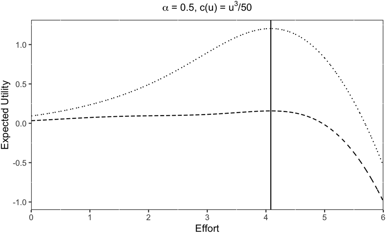
Plot of both player’s expected utility given that the respective opponent exerts equilibrium effort t when α = 0.5 and c(u) = u ³/50. The solid vertical line is placed at t. The dotted line represents player 1’s expected utility and the dashed line represents player 2’s expected utility.

However, this equilibrium easily breaks down when variables change slightly. If the head start α goes up to 0.6 the value of k* should be substantially increased to sustain the efficient level of effort. But at the same time, the upper bound on k would decrease with an increase in α, and at α = 0.6, k would not be below the upper bound anymore. Consequently, the equilibrium breaks down.

Changing the parameters of the cost function can also destroy the equilibrium. In fact, at the given values, lowering the cost of effort can lead to a violation of the second-order condition of player 2. If the cost function were given by c(u) = u ³/60, the value for c″((c′⁻¹(1))) would slightly decrease, leading the associated value of k* to increase so much, that player 2’s second-order condition is violated. The expected utilities are shown in Figure 2.

Figure 2:

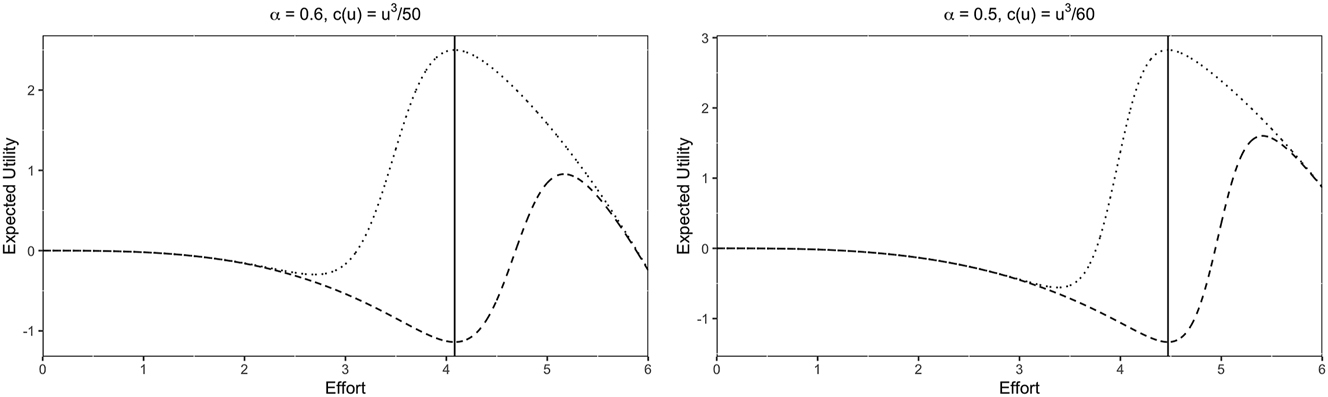
Plots of both players’ expected utility given that the respective opponent exerts the candidate equilibrium effort t where the equilibrium breaks down. For the first plot: α = 0.6 and c(u) = u ³/50 and for the second plot: α = 0.5 and c(u) = u ³/60. Again the solid vertical line is placed at t. The dotted line represents player 1’s expected utility and the dashed line represents player 2’s expected utility.

12 Discussion

In this section, we reconsider some assumptions regarding our modeling approach and show the robustness of our main results to these alternative specifications.

13 Conclusions

This paper examines contests with head starts and analyzes their impact on the incentives of players to exert effort. We have demonstrated that head starts can introduce distortions that prevent the implementation of efficient efforts in equilibrium. While a straightforward solution would be to use affirmative action to offset the effects of head starts, there are situations where affirmative action may be prohibited or not feasible. However, our analysis reveals that in the case of contests with only two players, the use of exponential Contest Success Functions (CSFs) enables the implementation of symmetric and efficient efforts in equilibrium.

References

Baye, M. R., and H. C. Hoppe. 2003. “The Strategic Equivalence of Rent-Seeking, Innovation, and Patent-Race Games.” Games and Economic Behavior 44: 217–26. https://doi.org/10.1016/s0899-8256(03)00027-7.Suche in Google Scholar
Calsamiglia, C., J. Franke, and P. Rey-Biel. 2013. “The Incentive Effects of Affirmative Action in a Real-Effort Tournament.” Journal of Public Economics 98: 15–31. https://doi.org/10.1016/j.jpubeco.2012.11.003.Suche in Google Scholar
Chen, B., X. Jiang, and D. Knyazev. 2016. Head Starts and Doomed Losers: Contest via Search. Available at SSRN 3067661.10.2139/ssrn.3067661Suche in Google Scholar
Denter, P., and D. Sisak. 2016. “Head Starts in Dynamic Tournaments?” Economics Letters 149: 94–7. https://doi.org/10.1016/j.econlet.2016.10.008.Suche in Google Scholar
Epstein, G. S., Y. Mealem, and S. Nitzan. 2013. “Lotteries vs. All-Pay Auctions in Fair and Biased Contests.” Economics & Politics 25: 48–60. https://doi.org/10.1111/ecpo.12003.Suche in Google Scholar
Feess, E., G. Muehlheusser, and M. Walzl. 2008. “Unfair Contests.” Journal of Economics 93: 267–91, https://doi.org/10.1007/s00712-007-0308-9.Suche in Google Scholar
Franke, J. 2012. “Affirmative Action in Contest Games.” European Journal of Political Economy 28: 105–18. https://doi.org/10.1016/j.ejpoleco.2011.07.002.Suche in Google Scholar
Franke, J., W. Leininger, and C. Wasser. 2018. “Optimal Favoritism in All-Pay Auctions and Lottery Contests.” European Economic Review 104: 22–37. https://doi.org/10.1016/j.euroecorev.2018.02.001.Suche in Google Scholar
Fu, Q. 2006. “A Theory of Affirmative Action in College Admissions.” Economic Inquiry 44: 420–8. https://doi.org/10.1093/ei/cbj020.Suche in Google Scholar
Hirshleifer, J. 1989. “Conflict and Rent-Seeking Success Functions: Ratio vs. Difference Models of Relative Success.” Public Choice 63: 101–12. https://doi.org/10.1007/bf00153394.Suche in Google Scholar
Jia, H. 2008. “A Stochastic Derivation of the Ratio Form of Contest Success Functions.” Public Choice 135: 125–30. https://doi.org/10.1007/s11127-007-9242-1.Suche in Google Scholar
Kirkegaard, R. 2012. “Favoritism in Asymmetric Contests: Head Starts and Handicaps.” Games and Economic Behavior 76: 226–48. https://doi.org/10.1016/j.geb.2012.04.005.Suche in Google Scholar
Knyazev, D. 2017. “Optimal Prize Structures in Elimination Contests.” Journal of Economic Behavior & Organization 139: 32–48. https://doi.org/10.1016/j.jebo.2017.04.017.Suche in Google Scholar
Laffont, J.-J., and D. Martimort. 2009. “The Theory of Incentives: The Principal-Agent Model.” In The Theory of Incentives. Princeton University Press.10.2307/j.ctv7h0rwrSuche in Google Scholar
Mealem, Y., and S. Nitzan. 2016. “Discrimination in Contests: A Survey.” Review of Economic Design 20: 145–72. https://doi.org/10.1007/s10058-016-0186-0.Suche in Google Scholar
Pelosse, Y. 2011. “Equivalence of Optimal Noisy-Ranking Contests and Tullock Contests.” Journal of Mathematical Economics 47: 740–8. https://doi.org/10.1016/j.jmateco.2011.10.005.Suche in Google Scholar
Schotter, A., and K. Weigelt. 1992. “Asymmetric Tournaments, Equal Opportunity Laws, and Affirmative Action: Some Experimental Results.” Quarterly Journal of Economics 107: 511–39. https://doi.org/10.2307/2118480.Suche in Google Scholar
Schweinzer, P., and E. Segev. 2012. “The Optimal Prize Structure of Symmetric Tullock Contests.” Public Choice 153: 69–82. https://doi.org/10.1007/s11127-011-9774-2.Suche in Google Scholar
Seel, C., and C. Wasser. 2014. “On Optimal Head Starts in All-Pay Auctions.” Economics Letters 124: 211–4. https://doi.org/10.1016/j.econlet.2014.05.018.Suche in Google Scholar
Siegel, R. 2014. “Asymmetric Contests with Head Starts and Nonmonotonic Costs.” American Economic Journal: Microeconomics 6: 59–105. https://doi.org/10.1257/mic.6.3.59.Suche in Google Scholar
Skaperdas, S. 1996. “Contest Success Functions.” Economic Theory 7: 283–90. https://doi.org/10.1007/bf01213906.Suche in Google Scholar
Szymanski, S. 2003. “The Economic Design of Sporting Contests.” Journal of Economic Literature 41: 1137–87. https://doi.org/10.1257/002205103771800004.Suche in Google Scholar
Tullock, G. 1980. “Efficient Rent Seeking.” In Toward a Theory of the Rent-Seeking Society, edited by J. M. Buchanan, R. D. Tollison, and G. Tullock, 97–112.Suche in Google Scholar
© 2024 the author(s), published by De Gruyter, Berlin/Boston
This work is licensed under the Creative Commons Attribution 4.0 International License.
Artikel in diesem Heft
- Frontmatter
- Research Articles
- Global Dynamics and Optimal Policy in the Ak Model with Anticipated Future Consumption