The Sobolev extension problem on trees and in the plane

1 Introduction

Let L m , p ( R n ) denote the homogeneous Sobolev space of real-valued functions on R n whose (distributional) derivatives of order m belong to L p ( R n ) for 1 < p < ∞. This space is equipped with the seminorm.

Provided p > n/m, any F ∈ L m , p ( R n ) is a continuous function, and therefore can be restricted to an arbitrary subset Ω ⊂ R n . We thus define the trace seminorm for functions f : Ω → R by

and we define the trace space L ^m,p (Ω) to be the set of all functions f : Ω → R with finite trace norm. We say that an operator T : L m , p ( Ω ) → L m , p ( R n ) is an extension operator if Tf|_Ω = f for every f ∈ L ^m,p (Ω).

In this article, we consider the Sobolev extension problem: Given a finite subset Ω ⊂ R n , does there exist a bounded linear extension operator T : L m , p ( Ω ) → L m , p ( R n ) satisfying ‖ T f ‖ L m , p ( R n ) ≤ C ‖ f ‖ L m , p ( Ω ) for some constant C = C(m, n, p) (in particular, C is independent of Ω)?

When p > n and m is arbitrary, the second-named author, C. Fefferman, and G.K. Luli [1] completely resolved this problem in the affirmative.

When n/m < p ≤ n, however, little is known. In this article, we consider the first nontrivial case in this parameter range – we study the Sobolev extension problem for the space L 2 , p ( R 2 ) when 1 < p < 2. (Note that the problem is well-understood when p = 2, because L 2,2 ( R 2 ) is a Hilbert space.) We refer to this as the planar Sobolev extension problem.

For the remainder of this article, we assume that 1 < p < 2. We now survey what is known about the planar Sobolev extension problem. (Our focus here is on the case in which the set Ω is finite; for interesting results when Ω is a bounded, simply connected domain, see [2].)

Recently, M. Drake, C. Fefferman, K. Ren, and A. Skorobogatova [3] showed that there is a bounded linear extension operator T : L 2 , p ( Ω ) → L 2 , p ( R 2 ) when Ω is a finite subset of a line in R 2 . Moreover, the norm of their extension operator depends only on p, as desired.

In our previous paper [4], we constructed a bounded linear extension operator T : L 2 , p ( Ω ) → L 2 , p ( R 2 ) for Ω belonging to a certain family of discrete subsets of R 2 with fractal geometry. We showed that the construction of such an operator could be reduced to an extension problem for a weighted Sobolev space on a tree. Thanks to a theorem of Fefferman–Klartag [5], we were able to solve the extension problem on the tree, and thus construct a linear extension operator for the Sobolev space on the plane.

In this article, we continue to investigate the connection between the planar Sobolev extension problem and weighted Sobolev extension problem on trees. The main theorem of this paper establishes conditions under which these problems are equivalent.

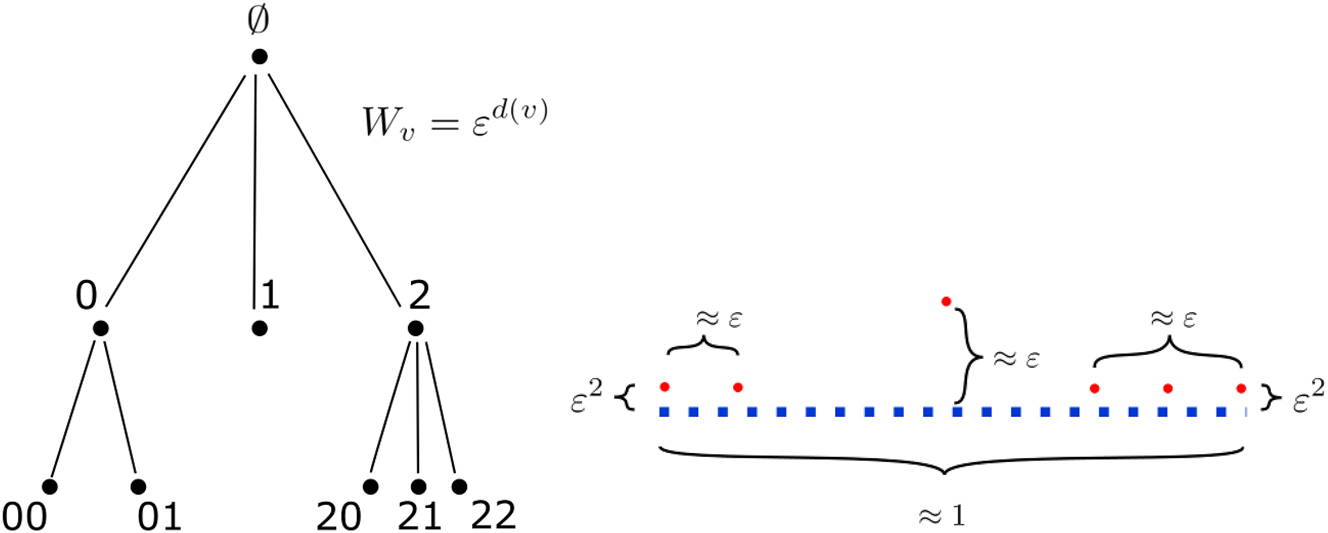
Consider a rooted N-ary tree of depth L ≥ 1 with vertices V. By N-ary, we mean that every non-leaf node has at most N children. In addition, to avoid degenerate branches, we require each non-leaf node to have at least 2 children. We’ll abuse notation and refer to V as the tree. We let d(v) denote the depth of v ∈ V.

We write [N] = {0, 1, … , N − 1}. We fix an ordering of the tree, i.e., an isomorphism from V to a subset of

so that any v ∈ V is identified with a string of d(v) digits from the set [N]. The root node of V is the empty string ∅ of length zero. Our convention above is that [N]⁰ = {∅}. We define V ₀ = V\{∅}.

For v ∈ V ₀ and 1 ≤ k ≤ d(v), let v _k denote the k-th entry of v and let π _k (v) ∈ V ₀ denote the prefix of v of length k. We define π ₀(v) = ∅ and write π(v) = π _d(v)−1(v) to denote the parent of v ∈ V ₀. We denote the set of leaves of V by ∂V.

Given vertices v ₀, v ₁ in V with d(v ₀) ≤ d(v ₁), if π d ( v 0 ) ( v 1 ) = v 0 then we say that v ₁ is a descendent of v ₀ and that v ₀ is an ancestor of v ₁. In particular, each vertex of V is both an ancestor and a descendent of itself. We let lca(x, y) denote the lowest common ancestor of x, y ∈ V, namely, the ancestor of x and y of largest depth.

We suppose that we are given a set of weights { W v } v ∈ V 0 , where W _v > 0 for every v ∈ V ₀. We define the L ^1,p (V)-seminorm of Φ : V → R by

and the L ^1,p (∂V) trace seminorm of ϕ : ∂ V → R by

We write L ^1,p (V), L ^1,p (∂V) to denote the vector spaces of real-valued functions on (respectively) V and ∂V with finite seminorm. We say that an operator H: L ^1,p (∂V) → L ^1,p (V) is an extension operator if Hϕ| _∂V = ϕ for all ϕ : ∂ V → R .

We now state the weighted Sobolev extension problem on trees: For any N-ary tree V, as above, does there exist a bounded linear extension operator H: L ^1,p (∂V) → L ^1,p (V) satisfying

for a constant C = C(p, N) (i.e., C is independent of V and the weights { W v } v ∈ V 0 )?

We say that an N-ary tree is perfect if each non-leaf node has exactly N children and all leaf nodes are at the same depth. We say that weights { W v } v ∈ V 0 are radially symmetric if W _v = W _u for every v, u ∈ V ₀ with d(v) = d(u).

Thanks to the work of Fefferman and Klartag [5] mentioned above, such an operator H is known to exist when V is a perfect, binary tree with radially symmetric weights. Additionally, in [6], A. Björn, J. Björn, J. Gill, and N. Shanmugalingam show that H can be taken to be a simple averaging operator when V is a perfect tree with radially symmetric weights satisfying certain additional properties. These are the only results that we are aware of on the problem of weighted Sobolev extension on trees. We emphasize that, to our knowledge, nothing is known for finite trees when either (1) the tree V is not perfect or (2) the weights are not radially symmetric.

In this article, we make neither of these assumptions. Instead, we introduce a parameter ɛ ∈ (0, 1) and say that weights { W v } v ∈ V 0 are radially decaying provided

Here and in the remainder of this paper, we adopt the convention that W _∅ = 1. Clearly, for such radially decaying weights we have

We then have the following theorem.

Thanks to Theorem 1, a negative answer to the problem of Sobolev extension on trees with radially decaying weights would resolve the planar Sobolev extension problem in the negative. This would be the first known example of a negative answer to the general Sobolev extension problem.

Alternatively, a positive answer to the problem of Sobolev extension on trees with radially decaying weights would produce the first known example of a bounded linear extension operator T : L 2 , p ( E ) → L 2 , p ( R 2 ) for certain sets E ⊂ R 2 .

We remark that we have made no attempt to compute the optimal value of the absolute constant k ₀ in Theorem 1, but taking, e.g., k ₀ = 10⁻¹⁰⁰ would certainly work.

For the remainder of this article we place ourselves in the setting of Theorem 1: We let k ₀ > 0 be a small enough absolute constant, to be picked later, and we fix an integer N ≥ 2, a rooted N-ary tree V (of which we fix some ordering), and radially decaying weights { W v } v ∈ V 0 satisfying (1) for some 0 < ɛ ≤ k ₀/N.

We now construct the set E ⊂ R 2 whose existence is asserted by Theorem 1. Define

and recursively define a map Ψ : V → R via

Observe that

The set E is then of the form

where

See Figure 1 for an illustration of E corresponding to a specific weighted tree of depth 2.

Figure 1:

A weighted tree V of depth 2 and the accompanying set E = E ₁ ∪ E ₂. Points of E ₁ are depicted by a sequence of blue squares of spacing ≈ ε 2 , while points of E ₂ are marked by 6 red dots.

We now comment briefly on the relationship between this work and our previous paper [4]. In that paper, we showed that for a certain set E ⊂ R 2 there exists a bounded linear extension operator L 2 , p ( E ) → L 2 , p ( R 2 ) if there exists a bounded linear extension operator L ^1,p (∂V) → L ^1,p (V) for a certain perfect, binary tree with radially symmetric decaying weights. Note that we did not prove the equivalence of these extension problems. The set E had the following geometric structure: It was the union of two sets, E 1 and E 2 . The set E 1 consisted of equispaced points on the x ⁽¹⁾-axis and the set E 2 was a truncated Cantor set contained in a line parallel to the x ⁽¹⁾-axis.

In the present paper, we are given an arbitary N-ary tree with radially decaying weights (not necessarily symmetric) and we produce a set E so that the relevant extension problems are equivalent. We remark that in the specific case of a perfect, binary tree with radially symmetric decaying weights (as in [4]), the set E will have the same geometric structure as the set E described above. In general, however, E will not be contained in the union of two parallel lines; see Figure 1 below.

In summary, the present paper improves the results of [4] by (1) establishing the equivalence of the extension problems and (2) allowing for far more general trees.

This concludes the introduction; the remainder of this article is devoted to the proof of Theorem 1.

We thank Marjorie Drake, Charles Fefferman, Bo’az Klartag, Kevin Ren, Pavel Shvartsman, Anna Skorobogatova, and Ignacio Uriarte–Tuero for helpful conversations. We also thank the anonymous referees for helpful feedback.

2 Preliminaries

Throughout this article, we will write K, K′, k, k′, … to denote positive absolute constants (independent of p, N, ɛ, and any other parameters we introduce), and K X , K X ′ , … to denote positive constants depending on a parameter X. The value of these constants may change from line to line. For A, B > 0 we write A ≲ B (resp. A ≲ _X B) if there exists a constant K (resp. K _X ) such that A ≤ KB (resp. A ≤ K _X B). We write A ≈ B (resp. A ˜  _X B) if A ≲ B and B ≲ A (resp. A ≲ _X B and B ≲ _X A).

Given δ > 0, we say a set S ⊂ R 2 is δ -separated provided |x − y|≥ δ for all distinct x, y ∈ S.

For a (possibly vector-valued) Lebesgue measurable function F defined on a measurable set S ⊂ R 2 with |S| > 0, we write (F) _S ≔|S|⁻¹ ∫ _S F dx.

Given an annulus A = x ∈ R 2 : r ≤ | x − x 0 | ≤ R with inner radius r and outer radius R, the thickness ratio of A is defined to be the quantity R/r.

The following version of the Sobolev inequality is proved in [4].

Let B(z, r) denote the ball of radius r > 0 centered at z ∈ R 2 , and let M denote the uncentered Hardy-Littlewood maximal operator, i.e.,

Recall that M is a bounded operator from L q ( R 2 ) to L q ( R 2 ) for any 1 < q ≤ ∞ (see, e.g., [7]).

Finally, we state as a lemma a simple fact about affine polynomials. We say that a triple of distinct non-colinear points x 1 , x 2 , x 3 ∈ R 2 are η-nondegenerate for η > 0 if |x _i − x _j |/|x _i − x _k | ≤ η ⁻¹ and ∠ ( x ⃗ i j , x ⃗ i k ) ≥ η for distinct i, j, k ∈ {1, 2, 3}; here, x ⃗ i j denotes the vector x _j − x _i and ∠(v, w) denotes the angle between vectors v , w ∈ R 2 .

3 Properties of the map Ψ

Recall the N-ary tree V fixed in Section 1. Note that the children of any vertex of V are ordered. Precisely, for children x, y of a common parent we say that x < y if x _d(x) < y _d(y).

This induces an ordering on the leaves ∂V. Consider distinct v, w ∈ ∂V with d(lca(v, w)) = m, so that v _i = w _i for all 0 ≤ i ≤ m but v _m+1 ≠ w _m+1. Then we say that v < w if and only if v _m+1 < w _m+1.

Recall that the map Ψ is used to define the set E ₂ in (7), and E 1 ⊂ R × { 0 } is defined in (6). We now establish some basic properties of the set E.

4 The Whitney decomposition

This section borrows heavily from Section 3 of our previous paper [4].

We will work with squares in R 2 ; by this we mean axis parallel squares of the form Q = [a ₁, b ₁) × [a ₂, b ₂). We let δ _Q denote the sidelength of such a square Q. To bisect a square Q is to partition Q into squares Q ₁, Q ₂, Q ₃, Q ₄, where δ Q i = δ Q / 2 for each i = 1, 2, 3, 4. We refer to the Q _i as the children of Q.

We define a square Q ⁰ = [−3, 5) × [−3, 5); note that E ⊂ Q ⁰. A dyadic square Q is one that arises from repeated bisection of Q ⁰. Every dyadic square Q ≠ Q ⁰ is the child of some square Q′; we call Q′ the parent of Q and denote this by (Q)⁺ = Q′.

We say that two dyadic square Q, Q′ touch if 1.1Q ∩ 1.1Q′ ≠ ∅. We write Q ↔ Q′ to denote that Q touches Q′.

For any dyadic square Q, we define a collection W ( Q ) , called the Whitney decomposition of Q, by setting

and

We write W = W ( Q 0 ) . Evidently, W is a partition of Q ⁰ by dyadic squares. Note that W ≠ { Q 0 } because #(3Q ⁰ ∩ E) = #E ≥ 2. We now collect a few useful properties of the family W .

We omit the proof of Lemma 5, as this type of decomposition is standard in the literature; see, e.g., [8].

Observe that property 2 of Lemma 5, combined with the fact that all dyadic squares arise from repeated bisection of Q ⁰, implies that for any Q , Q ′ ∈ W with Q ↔ Q′, we in fact have ∂Q ∩ ∂Q′ ≠ ∅.

We now remark that

To see this, observe that 3Q ⁺ ⊂ 9Q. Thus, Property 1 of Lemma 5 implies that #(9Q ∩ E) ≥ 2. Since the distance between distinct points of E is at least Δ, it follows that δ _Q ≥Δ/20, as claimed.

Let ∂Q denote the boundary of a square Q. We say that Q ∈ W is a boundary square if 1.1Q ∩ ∂Q ⁰ ≠ ∅. Denote the set of boundary squares by ∂ W . We remark that since dyadic squares arise from repeated bisection of Q ⁰, any boundary square Q ∈ ∂ W satisfies the stronger property Q ∩ ∂Q ⁰ ≠ ∅. Observe that

Indeed, this follows because E ⊂ [0, 2) × [0, 2), and if Q is a dyadic square intersecting the boundary of Q ⁰ = [−3, 5) × [−3, 5) with δ _Q ≤ 1/2, then Q ⁺ is a dyadic square intersecting the boundary of Q ⁰ with δ Q + ≤ 1 , which implies that 3Q ⁺ is disjoint from E, and hence Q ∉ W (see Part 1 of Lemma 4).

Note that

This follows from (13) and because E ⊂ [0, 2) × [0, 2), while Q ⊂ [−3, 5) × [−3, 5).

The collections W I , W I I , and W III form a partition of W because #(1.1Q ∩ E) ≤ 1 for any Q ∈ W , while the set E is partitioned as E = E ₁ ∪ E ₂. Also observe that

5 Clusters of the set E ₂

For the remainder of this article we fix a sufficiently large absolute constant K ₀ so that the conclusion of Lemma 7 holds. All constants K, k, etc. may depend on K ₀.

For each v ∈ V we define the shadow

Each shadow is a subset of ∂V; we let S = { S v } v ∈ V be the collection of shadows. Recall that we defined

and therefore the set of leaves ∂V is in one-to-one correspondence with the set E ₂. This determines an injection S → 2 E 2 (where 2 E 2 denotes the power set of E ₂). We define the cluster C _v ⊂ E ₂ to be the image of S _v under this injection, i.e.,

The set of all clusters

forms a tree under the relation of set inclusion, i.e., C ∈ C is an ancestor of C ′ ∈ C if C′ ⊂ C. Observe that for any two clusters C , C ′ ∈ C exactly one of the following is true: (1) C is an ancestor or descendant of C′, or (2) C ∩ C′ = ∅. We identify this tree with the tree V via the isomorphism v↦C _v . As with V, we denote the set of leaves of C by ∂ C = { C v } v ∈ ∂ V and we write C 0 = C \ { C ∅ } (note that C _∅ is the root node of the tree C ). The depth of a cluster in this tree is of course d(C _v ) = d(v) for v ∈ V.

We naturally associate to the tree C a family of weights { W C } C ∈ C by setting W C v = W v for every v ∈ V. We can then define the weighted Sobolev space L 1 , p ( C ) and the analogous trace space L 1 , p ( ∂ C ) . Since the weighted trees V and C are isomorphic, a bounded linear extension operator H: L ^1,p (∂V) → L ^1,p (V) induces a bounded linear extension operator H : L 1 , p ( ∂ C ) → L 1 , p ( C ) , and vice versa. Moreover, such operators have equal operator norms. We will make use of these facts in Sections 6 and 7.

We next detail some basic geometric properties of the clusters of E ₂.

Note that the root of the tree C is the set C _∅ = E ₂, while the set of leaves ∂ C is in one-to-one correspondence with the singleton sets of E ₂. Thus each C ∈ ∂ C is of the form C = {x _C } for a unique point x C = ( x C ( 1 ) , x C ( 2 ) ) ∈ E 2 . Observe that

Using Lemma 3, the definition of clusters (see (19), (20)), and the radial decay of the weights (recall, in particular, that ɛ < k ₀ N ⁻¹ < 1), we have

For each C ∈ C we fix a point y _C ∈ C. Observe that the singleton cluster {y _C } ⊂ E ₂ is contained in C. Thus, by (21), and the radial decay of the weights,

We let κ > 10 be a constant to be picked in a moment. Letting B ( x , r ) ⊂ R 2 denote the ball of radius r centered at x, we define

Here, K ₁ > 1 is a fixed absolute constant chosen so that

(see (22)); note that K ₁ does not depend on κ.

To prove (26), note that if C ∈ ∂ C then C is a singleton set, and y _C is the unique point of C. But y _C is the center of B _C , so C ⊂ κ ⁻¹ B _C . On the other hand, if C ∈ C \ ∂ C then diam(C) ≲ W _C by (22). Note that κ ⁻¹ B _C = B(y _C , K ₁ W _C ). Since y _C ∈ C, we have C ⊂ κ ⁻¹ B _C if K ₁ is large enough.

To prove (27), recall that C _∅ = E ₂ is the root of C and we have normalized the weights of the tree so that W E 2 = 1 . Then (27) is immediate provided that K ₁ is large enough.

Recall that the constant K ₀ > 1 was fixed at the beginning of this section, and recall the assumption that ɛ ≤ k ₀/N for a small enough constant k ₀. We claim that the family of balls { B C } C ∈ C has the following properties, provided κ is a large enough constant and k ₀ is sufficiently small depending on κ:

(B1) C ⊂ κ ⁻¹ B _C for every C ∈ C .

(B2) κB _C ⊂ B _π(C) for every C ∈ C 0 .

(B3) diam(B _C ) = 2K ₁ κW _C for every C ∈ C .

(B4) dist(K ₀ B _C , K ₀ B _C′) ≳ N ⁻¹(W _π(C) + W _π(C′)) for any C , C ′ ∈ C 0 with C ∩ C′ = ∅.

Properties (B1) and (B3) follow from (26) and (25), respectively. We prove properties (B2) and (B4) in a moment. First, however, observe that property (B4) implies:

(B5) The collection { K 0 B C } C ∈ ∂ C is pairwise disjoint.

(B6) For any ℓ ≥ 0 the collection

is pairwise disjoint (recall that d(C) denotes the depth of a node C in the tree C ).

(For the deduction of (B6) from (B4), note that clusters of identical depth are not ancestors or descendents of each other, and hence, must be disjoint.)

We now prove property (B2). Let C ∈ C 0 and y ∈ κB _C . Applying the triangle inequality, we get

Since C ⊂ π(C), we have y _π(C), y _C ∈ π(C) ⊂ κ ⁻¹ B _π(C) due to (B1). Therefore, by (B3),

Similarly, since y, y _C ∈ κB _C we have