
A Robust Factor Analysis Model for Dichotomous Data
-
Yixin Yang


Abstract
Factor analysis is widely used in psychology, sociology and economics, as an analytically tractable method of reducing the dimensionality of the data in multivariate statistical analysis. The classical factor analysis model in which the unobserved factor scores and errors are assumed to follow the normal distributions is often criticized because of its lack of robustness. This paper introduces a new robust factor analysis model for dichotomous data by using robust distributions such as multivariate t-distribution. After comparing the fitting results of the normal factor analysis model and the robust factor analysis model for dichotomous data, it can been seen that the robust factor analysis model can get more accurate analysis results in some cases, which indicates this model expands the application range and practical value of the factor analysis model.
1 Introduction
The classical factor analysis model is a powerful tool for exploratory data analysis or, more precisely, for reducing the dimensionality of the data. It is well known that factor analysis for category data is very common in psychological or medical investigations, and it also plays a very important role in economic analysis, market research as well as financial studies. Variables, such as gender and occupation, cannot appropriately be approximated by continuous distributions. Besides, some study of socio-economic status necessarily involves analyzing dichotomous data or data with a small number of categories.
This is not the first study about the factor analysis for categorical data. Some earlier works have been done, by some means or other, to treat categorical variables within the framework of the standard normal theory. Bock and Lieberman[1] originally proposed the item response theory (IRT). Christoffersson[2] studied the factor analysis (FA) of discretized variables. Muthén[3] extended the previous work. Although IRT and FA that cover similar types of categorical data differ in the tradition, the relationship between the two models is special as Bartholomew[4] alluded. Takane and De Leeuw[5] proved the equivalence of IRT and FA.
The classical factor analysis supposes that underlying factor scores and errors obey the normal distributions. However, the general maximum likelihood and Bayesian estimation under the normal distribution are not robust. There are some studies about the robust factor analysis model for continuous data. However, it is a pity that there is little similar work when the response variables are categorical or dichotomous particularly. In this paper we revisit and study in a deep-going way those previous studies on the factor analysis model for categorical data, which is called Item Response Theory (IRT) model. Then we will propose a robust factor analysis model for categorical data by expanding the original model and replacing the normal distribution assumption of unobserved factor scores by more robust distributions such as t-distribution. This paper will also perform the estimation of parameters as well as the methods of evaluating the model.
Numerical examples are given to show that the application of multivariate t-distribution not only significantly improves the robustness but also extends the application range and practical value.
2 Item Response Theory model
The approach in factor analysis for dichotomous data stems from the regression idea. To build an appropriate model for the regression of each yi which is a binary response on the latent variables, it is helpful to use logistic function for another use. It is reasonable to use the logistic function because of its theoretical and practical advantages. The logit model for binary data is one of the many item response models developed with Item Response Theory (IRT) approach. Bock and Moustaki[6] gave an overview of IRT regression models.
This IRT regression model can be adapted for the factor analysis. And a little literature focused on and introduced the building of the Item Response Theory model, which is a factor analysis model for dichotomous data with logistic idea. Baker and Kim[7], and van der Linden and Hambleton[8] considered to link the dichotomous manifest variables to a single latent variable through latent variable models.
We begin to revisit the related work by setting the problem in a general context and then introduce categorical data. The observed variables will be called manifest variables and are denoted by y = (y1, y2, ⋯ , yp)T. It is supposed in a latent structure model that these variables are associated to a set of unobservable latent variables denoted by f = (f1, f2, ⋯ , fq)T. And for the availability of the model, q needs to be much smaller than p. We can express the relationship between y and f by a conditional probability function p(y|f) that represents the distribution of y given f. This is a density or probability depends that y is continuous or categorical. Our aim is to acquire some information about the latent variables fs from the observed values of y. If h(f) denotes the joint distribution of the fs and f(y) denotes that of the ys, the relation between fs and ys will be presented by
After we have observed the values of y, the distribution of f is
In order to construct an available factor analysis model, there are some assumptions proposed. Firstly, an assumption that the fs are independent is imposed, that is
As a result, we can interpret and carry out the model in a easier way. The second assumption is about the form of p(fi). Although this distribution is essentially arbitrary, apparently, the choice may be suitable for our convenience. For this reason an extremely classical idea is that it follows a standard normal distribution.
The remaining work is to specify the function p(y|f). There is a crucial assumption about this function, which is fundamental to the principle of the method. Conditional independence is also a reasonable assumption, which is
This means that the observed correlation among the ys is wholly explained by their dependence on the fs. Given the underlying factors fs, the inter-dependence of the ys is eliminated. This is also a formal expression of the hypothesis that the observed variables are fully explained to the extent by a smaller number of latent dimensions.
For the application to contingency table we have introduced, initially, that each variable is dichotomous. Under this condition, we will write:
where pi(f) is the conditional probability of a response which is a positive response on the ith manifest variable.
Under the assumptions proposed above, the distribution of y can be derived as follows:
As pointed by Bartholomew (1980), there are some properties that the function pi(f) should possess, and it is natural to consider a class of functions given by
The coefficients αij are called “discrimination” coefficients, which can be interpreted as factor loadings. They also measure the extent to which the latent variable fj discriminates between individuals. The coefficient βi is the value of logit pi(f) at f = 0, which is called “difficulty” parameter. In practice such choices of G are limited, and the most commonly used function is the logit function or probit function.
In order to be more general, the conditional distribution of the complete p-dimensional response pattern can be specified as a function of the latent variables by adding the guessing parameter C. After given a random sample with p manifest variables of size n, we will get:
where m denotes the mth sample. The sample matrix is y = (ymi) and the ith manifest variable in the mth sample is denoted ymi which is a dichotomous manifest variable to be equal to 1 or 0. The vector of latent variables is denoted fm. Ci is the guessing parameter, αi is the discrimination parameter and βi is the difficulty parameter. g(·)is a logit function which is a link function map the range [–∞, ∞] to [0, 1], that is
For simplicity of the algorithm supporting the theory of this model, in practice, the guessing parameter is usually set as Ci = 0. And the total log-likelihood can be written as:
where h(f) is the density function of N(0, Ip), and pi denotes P(ymi = 1|fm).
3 Robust IRT model
People often criticize the normal factor analysis model because of its lack of robustness. The word “robustness” has different connotations in different cases. We use it in a relatively narrow sense: our goal is to establish a robust factor analysis model whose fitting result is acceptable, even if the standard normal assumptions are inaccuracy.
3.1 Building of the R-IRT model
A classical method to derive a useful extension when the model is built to analyze some smooth datasets is to use the t-distribution. This method is obtained in such a way that the maximum likelihood and the Bayesian estimation of the factor analysis model are calculated under the multivariate t-distribution[9, 10].
In the IRT model, there is an assumption of fm ∼ Np(0, Ip) for the mth sample. To improve the robustness of estimation, we shall replace the multivariate normal distribution of factor scores by the multivariate t-distribution. That is to say,
where νm denotes the multivariate t-distribution degrees-of-freedom for the mth sample. To be more convenient without losing reliability, it can be supposed that each νm is the same for every sample in this paper, which is denoted by ν.
Given a random sample with p manifest variables of size n, according to the classical IRT model, it is easy to know:
where m indicates the mth sample. The ith manifest variable in the mth sample is denoted by ymi which is a binary manifest variable to be equal to “1” or “0”. fm indicates the vector of latent variables. Ci is the guessing parameter. αi and βi are the discrimination parameter and the difficulty parameter respectively. g(·) is the logit link function, which is
Similarly, in most cases, we will assume each of the guessing parameter Ci = 0. If ym denotes the vector of responses for the mth sample unit. The total log-likelihood is:
where θ = (αi, βi). And pi = P(ymi = 1|f) indicates a conditional probability:
One matter should be pointed out is that fm here is assumed to follow tp(0, Ip, ν) and h(f) is the density function of tp(0, Ip, ν), where ν represents the multivariate t-distribution degrees-of-freedom.
It is available to estimate the parameters by maximizing the l(θ).
Factor scores are extremely important variables in factor analysis model. In this paper, an innovative method of estimating the factor scores which is derived from Bayesian idea will be presented, that is to use the mode of posterior distribution which is:
To explain how this Bayesian method can work, it need to be noticed that the posterior distribution of the factor scores can be derived given the mth sample ym. Having presented the assumptions and associated calculations, with regarding the estimated parameters as the real value of parameters here, the factor scores will be estimated by the software according to the following equation:
where h(f)is the density function of tp(0, Ip,ν) and
3.2 Evaluation of the model
Having fitted the model it is necessary to use some classical measures to evaluate the fitting results. Simplest, we can use the regression method to measure the fitting result. After making the regression line between O(r)and E(r) the model will tend to be regarded as an acceptable method qualitatively if the slope of the regression line is close to 1 enough.
An extremely classical and universal method is the goodness-of-fit test by comparing the observed and expected frequencies across the response patterns. That is, we prefer to use a χ2-statistic:
where O(r) and E(r) are the observed frequency and expected frequency of response pattern r respectively, and the summation is taken over all cells of the table. χ2 will have a χ2-distribution with degrees of freedom (2p – p(q +1) –1) approximately and we can judge the goodness of fit in this way[11].
Obviously,
There are 2p possible results for (y1, y2, ⋯ , yp) (yi=“0” or “1”), denoted by
Here two algorithms to calculate E(r) can be used in simulation process. In the first algorithm, we randomly generate T groups of numbers denoted by ft following a multivariate distribution tp(0, Ip, ν), which is similar to Monte Carlo method. Since t must be much bigger than 2p, we always supposed that T equals 1000 when p is less than 10 in our simulation, where p is the number of observed variables. The distribution of y on the condition of ft is written as:
Therefore,
The direct calculation is the second algorithm:
where h(f) is the density function of tp(0, Ip, ν). But because of the integration calculation, the time complexity of this algorithm is higher than the former one.
Since E(r) is the expected frequency of response pattern r, we estimate it by
After the calculation of the χ2 value, which is distributed approximately as chi-squared distribution with degrees of freedom (2p - p(q +1) – 1), the p value to check the goodness-of-fit can be achieved.
Up to now, this paper has accomplished the extension of IRT model to improve its robustness and building the R-IRT model.
4 Simulation
In this section, there are three different cases to be simulated in order to evaluate the proposed R-IRT model in this paper. The first data is from a classical educational test called the Law School Admission Test. The second example is to analyze a medical investigation data. To observe the performance of our R-IRT model further, the last part of this section will present the fitting results of the data generated according to the hypothesis of the model. All these three cases will show that the R-IRT model can improve the robustness of the factor analysis models as well as extend the application range of the factor analysis.
4.1 Case 1
In this subsection we will focus on a set of data from the Law School Admission Test (LSAT). LSAT is a classical case in educational testing for measuring ability traits presented in Bock and Lieberman[1] and the data are available in ltm, which is a R package, as the data.frame LSAT. For simplicity and without loss of generality, the data we use includes the responses of 1000 individuals to 3 questions, that is the first 3 columns data (n = 1000, p = 3).
The results of the “Mathematica” program which is to simulate what we have mentioned in this paper are presented as follows.
1. The analysis using the IRT model
It is an available way to get the estimations of parameters by maximizing the likelihood:
where pi = P(ymi = 1|f) = Ci + (1–Ci)g(αi1fm+βi), i = 1,2,3, and h(f) is the density function of N(0, 1). To be convenient, we set Ci = 0 for each of i, then pi = g(αi1fm + βi), i = 1,2,3.
The estimation results of related parameters are as follows.
The estimations of the parameters
| value | std | |
|---|---|---|
| α11 | –1.0065 | 0.0625 |
| α21 | –0.6794 | 0.1068 |
| α31 | –0.9808 | 0.0758 |
| β1 | 2.8883 | 0.2608 |
| β2 | 0.9777 | 0.1051 |
| β3 | 0.2552 | 0.0785 |
The coefficients {βi, i = 1,2,3} are “difficulty” parameters that are the value of logitpi(f) at f = 0. The coefficients {αi1} are “discrimination” coefficients, which can be interpreted in the usual way as factor loadings.
At the same time, the maximal likelihood is –1548.90.
The regression line between O(r)and E(r)are as the graph showing below:
The slope of the regression line between observed numbers and the expected numbers almost equals to 1, which reveals that the fitting result of the IRT model is acceptable.
To compare the different models further, we must do a more accurate and convincible test. The result of Global goodness-of-fit test is as follows:
Because there are 2p different categories of samples in the data and a kind of data corresponds to a sequence of scores, we can get the factor scores of the same quantity:
Factor scores of the size 2p for observed response patterns
| (y1, y2, y3) | factor score |
|---|---|
| (0,0,0) | 1.4039 |
| (0,0,1) | 0.7233 |
| (0,1,0) | 0.9333 |
| (0,1,1) | 0.2442 |
| (1,0,0) | 0.7053 |
| (1,0,1) | 0.0090 |
| (1,1,0) | 0.2258 |
| (1,1,1) | –0.4939 |
2. The analysis using the R-IRT model
As the scatter diagram showing above according to the original IRT model, the imitative effect is satisfactory to some extent. However the R-IRT model can improve it to a higher degree.
We set the degree-of-freedom of the multivariate t-distribution is 1, 5, 8 respectively, and the evaluation of fitting results is as the Table 3 showing.
The fitting results of the models for data LSAT
| Degree of the multivariate | The χ2 | p value of |
|---|---|---|
| t-distribution | value | the χ2 test |
| R-IRT: DF=1 | 4.348 | 0.037 |
| R-IRT: DF=5 | 0.014 | 0.904 |
| R-IRT: DF=8 | 0.061 | 0.804 |
| The original IRT | 0.198 | 0.656 |
Since there are at most 2p different categories of samples in the data, and a kind of data shares a set of scores, we can derive the factor scores of the size 2p when DF is 1, 5, 8 respectively with the method that has been proposed in this paper as the Table 4 showing below:
The factor scores of the size 2p for observed response patterns
| (y1, y2, y3) | DF=1 | DF=5 | DF=8 |
|---|---|---|---|
| (0,0,0) | –0.7646 | –1.2120 | –1.2894 |
| (0,0,1) | –0.2592 | –0.5428 | –0.6149 |
| (0,1,0) | –0.5125 | –0.7998 | –0.8510 |
| (0,1,1) | –0.0065 | –0.1282 | –0.1726 |
| (1,0,0) | –0.4504 | –0.6495 | –0.6723 |
| (1,0,1) | 0.0557 | 0.0243 | 0.0096 |
| (1,1,0) | –0.1980 | –0.2359 | –0.2307 |
| (1,1,1) | 0.3091 | 0.4480 | 0.4651 |
Though the result of fitting the classical IRT model is acceptable, as shown in the Table 3, the model using the multivariate t-distribution with 5-df performs better, as the p-value increases substantially to 0.904 compared with the original IRT model. And it can be observed that when the degree-of-freedom of the multivariate t-distribution in the R-IRT model continually increases, the result was closer to the p-value of the IRT model.
According to the results above, we can safely draw the conclusion that the robust IRT model can identify the latent factor of the manifest variables in LSAT data better comparing with the classical IRT model. That is to say, the R-IRT model achieves the purpose of reduction of the data dimension.
4.2 Case 2
The dataset that will be analyzed next has the responses of 89 individuals to 5 questions, which is from a medical investigation. These questions refer to whether individual has cerebral infarction, diabetes and hypertension or not. (n = 89, p = 3)
1. The analysis using the IRT model
Similarly, the estimations of parameters can be derived by maximizing the likelihood.
The maximal likelihood is –161.111.
The regression line between O(r) and E(r) are as the graph showing in Figure 2.
The estimations of the parameters
| value | std | |
|---|---|---|
| α11 | –1.9553 | 0.0963 |
| α21 | –1.8650 | 0.1500 |
| α31 | –0.6124 | 0.1490 |
| β1 | 1.6807 | 0.1691 |
| β2 | 0.6045 | 0.0694 |
| β3 | –0.7325 | 0.0821 |
Moreover, the result of Global goodness-of-fit test is as follows:
Similar with the previous example, the factor scores of the same quantity are as follows:
Factor scores of the size 2p for observed response patterns
| (y1, y2, y3) | Factor Score |
|---|---|
| (0,0,0) | 1.1517 |
| (0,0,1) | 0.9129 |
| (0,1,0) | 0.4579 |
| (0,1,1) | 0.2302 |
| (1,0,0) | 0.4250 |
| (1,0,1) | 0.1954 |
| (1,1,0) | –0.3511 |
| (1,1,1) | –0.6887 |
2. The analysis using the R-IRT model
The degree-of-freedom of the multivariate t-distribution is set as 1, 5, 8 respectively, and the evaluation of fitting results is as the Table 7 showing.
The fitting results of the models
| Degree of the multivariate | The χ2 | p value of |
|---|---|---|
| t-distribution | value | the χ2 test |
| R-IRT: DF=1 | 1.760 | 0.185 |
| R-IRT: DF=5 | 1.568 | 0.210 |
| R-IRT: DF=8 | 1.614 | 0.204 |
| The original IRT | 1.692 | 0.193 |
Similarly, the factor scores of the size 2p when DF is 1, 5, 8 respectively are presented as the Table 8 showing below:
The factor scores of the size 2p for observed response patterns
| (y1, y2, y3) | DF=1 | DF=5 | DF=8 |
|---|---|---|---|
| (0,0,0) | –1.1207 | –1.1728 | 0.6719 |
| (0,0,1) | –0.9205 | –0.9429 | 0.3521 |
| (0,1,0) | –0.4315 | –0.4666 | –0.2022 |
| (0,1,1) | –0.2230 | –0.2371 | –0.4336 |
| (1,0,0) | –0.4173 | –0.4370 | –0.2350 |
| (1,0,1) | –0.2085 | –0.2060 | –0.4648 |
| (1,1,0) | 0.3191 | 0.3518 | –0.9334 |
| (1,1,1) | 0.5503 | 0.6607 | –1.1670 |
Based on the simulation results of this data, it can be seen that the model using the multivariate t-distribution with 5-df performs best. But the advantage of the R-IRT model over the classical IRT model is not prominent. A possible reason is that the heavy tail effect of this set of data is not obvious, and the two model can obtain almost the same information.
4.3 Case 3
To evaluate the proposed model more theoretically, we generate a dataset according to the hypothesis of the R-IRT model in this subsection. That is to say, the data we will focus on satisfies the following distribution:
where f indicates the latent variables and f ∼tp(0, Ip, νm).
To be more specific, we generate fm ∼ t1 (0,1,3) randomly, and simulate a dataset {ymi} for i = 1, 2, 3 and m = 1,2, ⋯ ,1000.
The estimations of related parameters using maximizing the likelihood are as the Table 9 showing.
The estimations of the models
| The estimations | IRT model | R-IRT DF=1 | R-IRT DF=3 | R-IRT DF=5 |
|---|---|---|---|---|
| α11 | –1.2240(0.1082) | 0.6582(0.0568) | 0.9452(0.1136) | 1.1100(0.0963) |
| α21 | –0.9153(0.0720) | 0.4576(0.0535) | 0.6834(0.0484) | 0.8207(0.0766) |
| α31 | –1.3190(0.1834) | 0.7267(0.0533) | 1.0293(0.1094) | 1.2004(0.1340) |
| β1 | 0.3895(0.0326) | 0.3930(0.0376) | 0.3921(0.0320) | 0.3907(0.0297) |
| β2 | 0.4226(0.0255) | 0.4270(0.0398) | 0.4256(0.0339) | 0.4239(0.0306) |
| β3 | 0.4284(0.0517) | 0.4320(0.0383) | 0.4311(0.0483) | 0.4296(0.0577) |
The results of Global goodness-of-fit tests of the IRT model and the R-IRT model are as the Table 10 showing.
The fitting results of the models
| Degree of the multivariate t-distribution | The χ2 value | p value of the χ2 test |
|---|---|---|
| R-IRT: DF=1 | 5.114 | 0.023 |
| R-IRT: DF=5 | 1.426 | 0.232 |
| R-IRT: DF=8 | 1.923 | 0.166 |
| The original IRT | 2.250 | 0.134 |
In the meanwhile, the factor scores in the IRT model and the R-IRT model are as follows in Table 11.
The factor scores of the size 2p for observed response patterns
| (y1, y2, y3) | IRT model | R-IRT with DF=1 | R-IRT with DF=3 | R-IRT with DF=5 |
|---|---|---|---|---|
| (0,0,0) | 1.0545 | 0.5778 | 0.6921 | 0.7298 |
| (0,0,1) | 0.3801 | 0.0041 | 0.0173 | 0.0252 |
| (0,1,0) | 0.5809 | 0.2151 | 0.2385 | 0.2393 |
| (0,1,1) | –0.07782 | –0.3518 | –0.4112 | –0.4247 |
| (1,0,0) | 0.4272 | 0.0577 | 0.0707 | 0.0757 |
| (1,0,1) | –0.2376 | –0.5071 | –0.5744 | –0.5826 |
| (1,1,0) | –0.0294 | –0.2987 | –0.3588 | –0.3753 |
| (1,1,1) | –0.7470 | –0.8613 | –1.0052 | –1.0421 |
After a comparison between the p-values of the IRT model and the R-IRT model, we can observe the R-IRT model using the multivariate t-distribution with 3-df performs best. Although the overall imitative results are not very satisfactory, which may be caused by the shrink of the sample information, the applicability and advantages of the R-IRT model are still performed.
4.4 Analysis on the results of fitting
Though the results of fitting the original IRT model may be reluctantly acceptable, as shown in the Figure 1 and Figure 2, the model using the multivariate t-distribution performs better, especially with a medium degree of freedom. The reason for it may be that quality of the t-distribution with a medium degree of freedom is between quality of the normal distribution and quality of the t-distribution with 1-df, which leads to the model has more excellent properties. Besides, when the degree-of-freedom of the multivariate t-distribution in the R-IRT model continually increases, the p-value was closer to that of the IRT model.
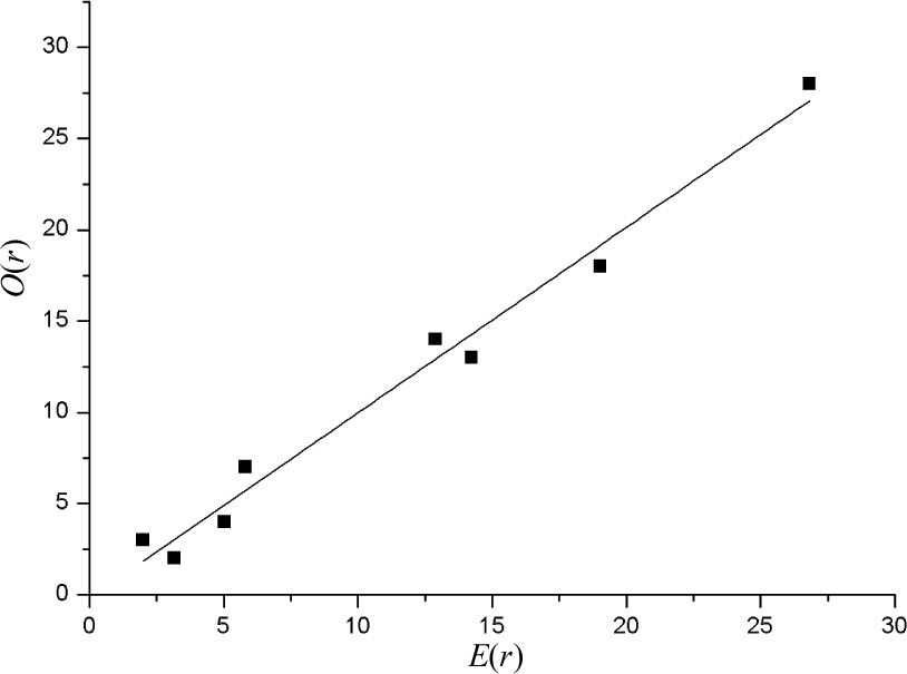
The relationship between O(r)and E(r)in the IRT model
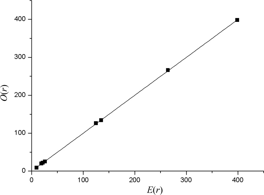
The relationship between O(r) and E(r) in the IRT model
According to the comparison between the p-values of the IRT model and the R-IRT model, the advantage of the later one has been found. To analyze theoretically, it can be easily understood. Since multivariate t-distribution is called to be the typical “Heavy-Tailed Distribution”, the robust model can get more information and describe more features of the data. All the reasons above explain why the R-IRT model performs better.
5 Conclusion
Factor analysis model is a classical way to reduce the dimensionality of the data. Unfortunately, there were only a few insufficient studies about the factor analysis for categorical data before. Towards solving the limitation issue in the classical factor analysis, this paper proposes a robust method of factor analysis for dichotomous data. This R-IRT model is obtained from the original IRT model by replacing the normal distribution with the multivariate t-distribution. At the same time, the estimations of some crucial parameters and variables such as score factors are successfully derived in this paper.
According to the simulations presented, it can be seen that in a great many cases, the R-IRT model for dichotomous data is more efficient and acceptable than the original IRT model. It shows that the application of multivariate t-distribution not only significantly improves the robustness of the factor analysis models but also extends the application range and practical value of the models. And when the distributions of factor scores become smooth, we may hardly expect the original model under the hypothesis of the normality distribution to help us find the latent information by a small amount of dimensions effectively.
An effective simulation using “Mathematica” software is accomplished, but there are still some challenges to be faced with in the research process. An important shortcoming is that, we cannot fit the models efficiently when the factor dimension q is big enough because of the complexity of the algorithm. The algorithm needs to be accelerated as the sample dimension p or the factor dimension q increases.
References
[1] Bock R D, Lieberman M. Fitting a response model for n dichotomously scored items. Psychometrika, 1970, 35(2): 179–197.10.1007/BF02291262Suche in Google Scholar
[2] Christoffersson A. Factor analysis of dichotomized variables. Psychometrika, 1975, 40(1): 5–32.10.1007/BF02291477Suche in Google Scholar
[3] Muthén B. Contributions to factor analysis of dichotomous variables. Psychometrika, 1978, 43(4): 551–560.10.1007/BF02293813Suche in Google Scholar
[4] Bartholomew D J. Factor analysis for categorical data. Journal of the Royal Statistical Society, Series B, 1980, 42(3): 293–321.10.1111/j.2517-6161.1980.tb01128.xSuche in Google Scholar
[5] Takane Y, De Leeuw J. On the relationship between item response theory and factor analysis of discretized variables. Psychometrika, 1987, 52(3): 393–408.10.1007/BF02294363Suche in Google Scholar
[6] Bock R D, Moustaki I. Item response theory in a general framework. Handbook of Statistics: Psychometrics, 2007, 26: 469–513.10.1016/S0169-7161(06)26015-2Suche in Google Scholar
[7] Baker F B, Kim S H. Item response theory: Parameter estimation techniques. CRC Press, New York, 2004.10.1201/9781482276725Suche in Google Scholar
[8] van der Linden W J, Hambleton R K. Handbook of modern item response theory. Springer, New York, 1997.10.1007/978-1-4757-2691-6Suche in Google Scholar
[9] Li J, Liu C, Zhang J. Robust factor analysis using the multivariate t-distribution. Metrica, 2007, 29: 178– 181.Suche in Google Scholar
[10] Lange K L, Little R J A, Taylor J M G. Robust statistical modeling using the t-distribution. Journal of the American Statistical Association, 1989, 84(408): 881–896.10.2307/2290063Suche in Google Scholar
[11] Bartholomew D J, Leung S O. A goodness of fit test for sparse 2p contingency tables. British Journal of Mathematical and Statistical Psychology, 2002, 55(1): 1–15.10.1348/000711002159617Suche in Google Scholar PubMed
[12] Bartholomew D J. Latent variable models for ordered categorical data. Journal of Econometrics, 1983, 22(1): 229–243.10.1016/0304-4076(83)90101-XSuche in Google Scholar
[13] Knott M, Bartholomew D J. Latent variable models and factor analysis. Edward Arnold, London, 1999.Suche in Google Scholar
[14] Agresti A. Categorical data analysis. John Wiley & Sons, New York, 2002.10.1002/0471249688Suche in Google Scholar
[15] Heinen T. Latent class and discrete latent trait models: Similarities and differences. Sage Publications Inc, New York, 1996.Suche in Google Scholar
[16] Harman H H. Modern factor analysis. University of Chicago Press, Chicago, 1976.Suche in Google Scholar
[17] Kolenikov S, Angeles G. Socioeconomic status measurement with discrete proxy variables: Is principal component analysis a reliable answer? Review of Income and Wealth, 2009, 55(1): 128–165.10.1111/j.1475-4991.2008.00309.xSuche in Google Scholar
[18] Hambleton R K, Swaminathan H, Rogers H J. Fundamentals of item response theory. Sage, New York, 1991.Suche in Google Scholar
[19] Lord F M, Novick M R. Statistical theories of mental test scores. Reading, MA: Addison, 1968.Suche in Google Scholar
[20] McDonald R P. The common factor analysis of multicategory data. British Journal of Mathematical and Statistical Psychology, 1969, 22(2): 165–175.10.1111/j.2044-8317.1969.tb00428.xSuche in Google Scholar
[21] Plackett R L, Stuart A. The analysis of categorical data. Griffin, London, 1974.Suche in Google Scholar
[22] Knott M, Bartholomew D J. Latent variable models and factor analysis. Edward Arnold, London, 1999.Suche in Google Scholar
[23] Kamata A, Bauer D J. A note on the relation between factor analytic and item response theory models. Structural Equation Modeling, 2008, 15(1): 136–153.10.1080/10705510701758406Suche in Google Scholar
[24] Relles D A, Rogers W H. Statisticians are fairly robust estimators of location. Journal of the American Statistical Association, 1977, 72(357): 107–111.10.1080/01621459.1977.10479918Suche in Google Scholar
[25] Yuan K H, Chan W, Bentler P M. Robust transformation with applications to structural equation modelling. British Journal of Mathematical and Statistical Psychology, 2000, 53(1): 31–50.10.1348/000711000159169Suche in Google Scholar PubMed
[26] Rizopoulos D. LTM: An R package for latent variable modeling and item response theory analyses. Journal of Statistical Software, 2006, 17(5): 1–25.10.18637/jss.v017.i05Suche in Google Scholar
[27] R Development Core Team. R: A language and environment for statistical computing. R Foundation for Statistical Computing, Vienna, Austria, 2006. Available at http://www.R-project.org.Suche in Google Scholar
© 2014 Walter de Gruyter GmbH, Berlin/Boston
Artikel in diesem Heft
- Spatial Dynamics, Vocational Education and Chinese Economic Growth
- The Differential Algorithm for American Put Option with Transaction Costs under CEV Model
- Nonlinear Dynamics of International Gold Prices: Conditional Heteroskedasticity or Chaos?
- Design and Pricing of Chinese Contingent Convertible Bonds
- A Robust Factor Analysis Model for Dichotomous Data
- Non-linear Integer Programming Model and Algorithms for Connected p-facility Location Problem
- Uncertain Comprehensive Evaluation Method Based on Expected Value
- MSVM Recognition Model for Dynamic Process Abnormal Pattern Based on Multi-Kernel Functions