Galilean decoherence and quantum measurement

2.1 General remarks

We begin with a few remarks that somewhat soften the supposed contrast between “individual system interpretation” and “ensemble interpretation” of quantum states. In doing so, we emphasize the differences to classical theories, for which we consider classical statistical mechanics (CSM) as a generic example. Thereby we ignore mathematical subtleties that are irrelevant to this discussion. For example, pure states in CSM would be represented mathematically by points in phase space, whereas in any physical application finite uncertainty arises. Realistically, pure states are not realized by delta functions on phase space but approximated by functions with a finite width.

First, we consider pure states in quantum theory that are represented by projectors P = |ψ⟩⟨ψ| in a Hilbert space H with ψ ∈ H and ψ = 1 . If an ensemble of individual systems is prepared in a pure state P, it is permitted to assign this pure state P to each system S of the ensemble in the sense that any subsequent measurement on S cannot lead to a contradiction to this assignment. For example, a yes-no measurement with the projector P will definitely return the result “yes” (or “1”) while another yes-no measurement with a projector Q ⊥ P would return the result “no” (or “0”) with certainty. All other yes-no measurements can result in “1” or “0” without the possibility of predicting the outcome. The difference to the CSM is that the existence of a pure state for an individual system is not only a permissible assumption here, but can also be fully verified by a single test measurement. In quantum mechanics no single measurement can detect a pure state without using additional information, see, e.g., [17] §9.4.

Next, we consider genuinely mixed states, which are represented mathematically by statistical operators W in the Hilbert space H , excluding the case W = P. Here we have to distinguish between “proper mixtures” and “improper mixtures”. For proper mixtures, a partition of the corresponding ensemble into sub-ensembles corresponding to pure states P _i , satisfying W = ∑ _i p _i P _i , can be distinguished due to the closer circumstances. Again, it is allowed to assume that each individual system S of the ensemble corresponding to W “has” one of the states P _i , but one does not know which one (“ignorance interpretation”). This assumption cannot lead to a contradiction with the result of a subsequent measurement. For example, in the case of mutually orthogonal P _i , a measurement of an observable with the eigenprojectors P _i will give the result which of the pure states P _i can be assigned to S, and is hence consistent with the assumption. In CSM the situation is similar except that the partition of the ensemble into pure states is unique and need not be given as an additional information for the test measurement.

In the case of improper mixtures, it is not possible to distinguish such a decomposition of the ensemble depending on the closer circumstances. Below we will give an example where an assignment of pure states to individual systems of the ensemble can even be ruled out. In CSM the case of improper mixtures does not occur since the decomposition of a mixed state into pure states is always unique.

The announced example consists of the EPR-experiment, where a pair of particles is prepared in an entangled, rotationally invariant spin state 1 2 ( ↑ ↓ − ↓ ↑ ) so that one particle is sent to Alice and the other one to Bob. If Alice makes a measurement of the spin into direction a, corresponding to the observable (Hermitean operator) A = a ⋅ σ , the probability of “spin up” will be 1/2 regardless of the direction a. Hence Alice will find that her particle has a mixed spin state described by W = 1 2 1 | . The same applies to Bob. Whether W represents a proper or an improper mixture depends on the circumstances of the experiment.

If Bob has made a spin measurement of the observable B = b ⋅ σ then it would be legitimate to call the mixed state W of the particle sent to Alice “proper” and the corresponding decomposition W = ∑ _i p _i P _i is given by the two eigenprojectors P_↑, P_↓ of B, with p_↑ = p_↓ = 1/2. According to the above it would be permissible to assume that each particle arriving at Alice “has” either spin up or spin down w.r.t. the direction b chosen by Bob and corresponding to the perfect anti-correlation of spin measurement results of Alice and Bob.

The situation is different in the case where Bob has not made any spin measurement. Although the particles sent to Alice are characterized by the same mixed state W = 1 2 1 | as before, this mixture has now to be classified as “improper”. Imagine that Alice adopts a “double ignorance interpretation” in the sense that she assumes a proper mixture of the form W _A = p_↑P_↑ + p_↓P_↓, but without knowing the direction of ↑. The analogous assumption will be made by Bob. To account for the anti-correlations as much as possible, Bob should choose the same unknown spin direction as Alice. Both assumptions can be combined so that, taking into account the anti-correlation, the overall state has the form W ̃ = 1 2 P ↑ ↓ + 1 2 P ↓ ↑ . This results in a mixture of product states for the combined system, which is different from the pure state given by the projector V on 1 2 ( ↑ ↓ − ↓ ↑ ) . However, the difference between V and W ̃ with unknown direction of ↑ cannot be detected by a single measurement, but only by a long series of measurements.

We conclude that the “individual system interpretation” of quantum states is possible in some cases, namely for pure states and proper mixtures, but for the general case, including improper mixtures, the “ensemble interpretation” is indispensable. In this respect, our argument goes beyond Ballentine [13], who sees in the “individual system interpretation” a conceivable but superfluous supplement to the “ensemble interpretation”, against which, among other things, Ockham’s razor argument speaks.

2.2 Preparation and registration procedures

We have seen in the preceding subsection that the distinction between “proper” and “improper” mixtures cannot be made at the level of statistical operators W but depends on the “closer circumstances” of the experiments. This can be taken as a motivation for introducing a refined vocabulary: A state described by W is not represented by a single ensemble of identically prepared systems but by a class of ensembles corresponding to different “preparation procedures”. Such a refined theory has been elaborated by Ludwig [15] and need not be reproduced here in all details. We will focus on the aspects relevant to this paper.

The attempt to interpret a quantum mechanical state as a single ensemble E of quantum systems leads to another problem: Every conceivable measurement of an observable (Hermitian operator) A, which has a complete system of eigenprojectors, leads to a corresponding partition of E consisting of subsets of E where the observable A has a definite value. For arbitrary finite sets of non-commuting observables and a dimension of the Hilbert space ≥ 3 , however, the existence of these partitions of a single ensemble E leads to a contradiction according to the theorem of Kochen and Specker [18].

A characteristic feature of Ludwig’s approach is the extension to preparation and registration procedures. Both types of procedures contain the description or construction manual of macroscopic devices in a classical language and can be realized by concrete processes as often as required. A single experiment consists of a combination of a realization of a preparation procedure and of a registration procedure and can be in turn be repeated as often as you want. The problem arises that there are obviously different combinations that differ in the relative spatio-temporal position of their parts. Ludwig solves this problem by demanding that the construction manuals refer to an abstract coordinate frame, which is replaced by a concrete coordinate frame for each realization. If you combine a preparation procedure and a registration procedure, you only need to identify the abstract coordinate frames. Another advantage of the introduction of abstract coordinate frames is that it enables a natural definition of time-translations or, more general Galilei transformations, operating on the coordinate frames of preparation procedures (Schrödinger picture) or, alternatively, of registration procedures (Heisenberg picture).

The purpose of an experiment is to obtain results. Ludwig’s formalism takes this aspect into account by assigning a probability λ(a, b₀, b) to the triple of a preparation procedure a, a registration procedure b₀ and an event b that can occur during the measurement. This leads to a function μ : Q × F → [ 0,1 ] , where Q is the set of (non-empty) preparation procedures and F the set of “effect processes” consisting of pairs (b₀, b) and describing generalized yes-no measurements. Different events b _i for the same registration procedure b give rise to “coexistent effect processes”. Each preparation procedure therefore induces a real function defined on F , but two different preparation procedures can induce the same function. Proceeding to the corresponding equivalence classes of preparation procedures, one obtains “states” (we have avoided Ludwig’s notion of “ensembles” as it could be confused with the previously discussed concept). Analogously, one considers “effects” as equivalence classes of statistically equivalent effect processes, and a derived probability function

where K denotes the set of states and L the set of effects. Coexistent effect processes generate “coexistent effects”. In his work [15] Ludwig further provides physical axioms for the structure (K, L, μ) such that K can be represented as the set of statistical operators W on a Hilbert space H and L as the set of Hermitean operators F on H such that 0 ≤ F ≤ 1 | and the statistical function μ is represented as Tr(WF).

The description of a particular experiment with the terms developed by Ludwig can sometimes be done in different ways, which is reminiscent of the shiftability of the cut in the Copenhagen interpretation. Consider, for example, the EPR experiment mentioned in the Section 2.1 of two measurements of Alice and Bob, resp., on a pair of particles. On the one hand, these measurements can be understood as coexistent effects measured for a pure state given by the projector onto 1 2 ( ↑ ↓ − ↓ ↑ ) . On the other hand, the preparation of the entangled pair together with the measurement of Bob can be understood as the preparation a of a mixed state W = 1 2 1 | on which Alice performs a measurement. The decomposition of the set of individual systems prepared according to a, corresponding to the result “yes” or “no” of Bob’s measurement, can be understood as a decomposition of a into two partial preparation procedures, a = a₁ ∪ a₂, which further leads to the convex linear combination W = 1 2 P ↑ + 1 2 P ↓ at the level of the states. We have referred to this as a “proper mixture” in Section 2.1.

2.3 Ensemble interpretation and the measurement problem

To fix the notation we will assume that, after the interaction between the microsystem and the measurement apparatus, the total system assumes the pure state

where the states |Ψ _α ⟩ refer to the microsystem and the states |ψ _α ⟩ to the various outcomes which can be read off the measurement apparatus. Ballentine has argued [13] that this only then contradicts the experience that the measuring apparatus shows an unambiguous result if one assumes the individual system interpretation for the pure state Φ. There is supposedly no such problem with the ensemble interpretation for Φ.

We will discuss this position using Ludwig’s elaboration of the ensemble interpretation outlined in the last subsection. Then the state Φ is realized by a preparation procedure a. One could of course object that the preparation of a pure initial state for the measuring apparatus, which leads to (2) after time t, is extremely unrealistic. But this would be an argument against Q-monism. The discussion we analyze here, however, takes place within the framework of Q-monism, and is thus based on the premise that such a preparation procedure a is conceivable.

In Ludwig’s language, the states ψ _α of the measuring apparatus can be interpreted as mutually exclusive coexistent effect processes, which enable a disjoint decomposition of the preparation procedure a of the form a = ⋃ _α a _α , similar to the EPR example from the Section 2.2. But this would result in a mixed state Φ, in contradiction to the assumption that Φ is a pure state.

We therefore come to the conclusion that the measurement problem persists, regardless of the interpretation of the state Φ according to the individual system interpretation or the ensemble interpetation.

3.1 Definitions

We consider non-relativistic quantum theory based on Galilean space-time M which is assumed to be a 4-dimensional affine space. Let G denote the (proper) Galilei group acting on M by means of affine bijections g : M → M , g ∈ G . W.r.t. a fixed Galilean coordinate system γ : M → R × R 3 , γ ( m ) = ( t , x ) , Galilean transformations can be identified with the quadruple g = ( b , a , u , R ) ∈ R × R 3 × R 3 × S O 3 such that

The connection to quantum theory is given by a projective, unitary, irreducible representation (“irrep”) R of G . This representation is characterized by a positive real number m (“mass”), a positive half-integer number s (“spin”), and a Hilbert space

such that

see, for example, [19], [20]. Here E = p 2 2 m and D ^s is the (2s + 1)-dimensional projective, unitary irrep of SO₃ or, equivalently, the (2s + 1)-dimensional unitary irrep of SU₂.

For the following we neglect the rotational degrees of freedom and thus set s = 0. Time translations are not considered since they correspond to a free time evolution and we will instead consider a more general unitary, Galilei invariant time evolution U(t). Moreover, for the purposes of this paper it will be convenient to pass from the momentum representation to the velocity representation of wave functions and hence to consider the Hilbert space

Then (5) will be reduced to

where ψ ∈ H ̂ m . In the position representation of wave functions obtained by an inverse Fourier transformation we use the Hilbert space

Explicitly, the transformation from ϕ ∈ H m to ψ ∈ H ̂ m can be written as

Then we obtain the positional representation of the reduced Galilean irrep analogous to (7) (denoted by the same letter)

where ϕ ∈ H m .

3.2 Postulates and first results

So far, we have only sketched the well-known form of non-relativistic quantum theory. We will modify this theory by postulating that the “pure” time evolution described by a unitary family U(t) that commutes with the reduced Galilean irrep (10) is superimposed by a global quantum fluctuation:

The distribution of the two random variables a and u is left open, except that it is identical for all intervals (t, t + δt) and will be later restricted by certain assumptions on its statistical parameters. The order of space translations and boosts is irrelevant since, according to Weyl’s commutation relation, the commutator of their irreps is a constant phase factor that cancels if calculating probabilities.

We will discuss the consequences of Postulate 1 for the statistical interpretation of quantum theory, as outlined in Section 2.2. We will concentrate on the influence of random translations and boosts on the ensemble W, since the pure time evolution commutes with their representation. For two different time intervals (t₁, t₁ + δt) and (t₂, t₂ + δt) the values of the random variables a and u and their irreps R ( 0 , a , u , 1 | ) will be different. But due to the statistical interpretation of the state W the individual Galilean fluctuations are not important but only the mean value of the corresponding irreps over many time intervals (t, t + δt). Additionally we use the assumption δt ≪ Δt to invoke the central limit theorem. Let Δt = Nδt with a large integer N then the sum of N random spatial translations and boosts has asymptotically a normal distribution with mean values and variances proportional to N and hence to Δt. The mean values of a and u are assumed to vanish. This leads to the modified Postulate

In the language of stochastic processes we thus assume that a _t and u _t are independent 3-dimensional Brownian motions with variances σ²(a _t − a _s ) = α (t − s) and σ²(u _t − u _s ) = β (t − s) for s < t, resp., see, e.g., Def. 2.1 in [21]. In other words, the components of a _t and u _t are Lévy processes with vanishing jump term in the Lévy-Khintchine formula, cf. theorem (42.6) in [21].

In order to calculate the effect W ↦ W ′ = T S W of the spatial quantum fluctuations a on the statistical operator W we assume its velocity representation by means of the integral kernel W(v, w). According to Postulate 1 and (7) we obtain

Note that the transformation W ↦ W ′ = T S W preserves positivity and trace, and hence maps statistical operators onto statistical operators, although it is not unitarily induced. Being a mixture of unitarily induced transformations it is completely positive [22] and, moreover, increases the von Neumann entropy S(W) = −k _B Tr(W logW) since W ↦ S(W) is a concave function.

It will be convenient to introduce new velocity coordinates by

and to rewrite (14) in the form

Analogously, we calculate the effect W ′ ↦ W ′ ′ = T B W ′ of the quantum boost fluctuations u on the statistical operator W′ in terms of its position representation given by the integral kernel W′(x, y) and using (10):

Also this result will be rewritten by introducing new position coordinates

and assumes the form

Due to the similar structure also the transformation W ′ ↦ W ′ ′ = T B W ′ preserves positivity and trace, is completely positive and implies an increase of von Neumann entropy. This underlines the dissipative character of the modification of the unitary time development that we are looking at.

Differentiating (18) w.r.t. the time parameter Δt gives the term − m 2 β 2 ℏ 2 ( x − y ) 2 W ′ ′ ( x , y ) to be compared with the term − λ ρ ( t ) − T [ ρ ( t ) ] in eq. (3.1) of [10], where the position representation of the localization operator T is given in eq. (2.10). This shows that, despite some similarities, our ansatz differs significantly from the GRW approach, and not only with respect to individual system versus ensemble interpretation of quantum states.

For later purposes we will prove the following

3.3 Illustration of decoherence effects

It is plausible that the damping of the “off-diagonal” regions of the integral kernels W(v, w) and W′(x, y) by the transformations (14) and (18) possibly leads to decoherence effects. Nevertheless, it will be instructive to study these effects by means of an example.

We consider only one spatial dimension x and a statistical operator W′ with integral kernel W′(x, y) given by the projector onto a wave function representing a superposition of two wave functions sharply localized at x = A and x = B, resp., such that A < B. It follows that W′(x, y) almost vanishes everywhere except for four small regions located around the points (x = A, y = A), (x = A, y = B), (x = B, y = A) and (x = B, y = B), see Figure 1. Through the transformation W′ ↦ W″, see (18), the integral kernel W′(x, y) is multiplied by the “damping” Gaussian exp − m 2 β Δ t 2 ℏ 2 ( x − y ) 2 which has the width

in the η-direction orthogonal to the diagonal x = y.

Figure 1:

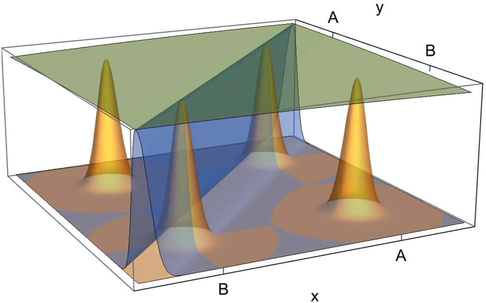
Illustration of decoherence effects. The integral kernel W′(x, y) (dark yellow surface) corresponds to a wave function that is strongly concentrated at the points x = A and x = B. By multiplication with a Gaussian damping function that fulfills the condition Δη ≪ |A − B| (blue surface), where Δη is the width of the Gaussian in the direction orthogonal to the diagonal x = y, defined in (23), the off-diagonal peaks of W′(x, y) are suppressed. In contrast, multiplication with a Gaussian damping function that satisfies Δη ≫ |A − B| (green surface) leaves W′(x, y) practically unchanged.

The effect of this multiplication depends on the size of Δη relative to |A − B|: If Δη ≫ |A − B| the integral kernel W′(x, y) remains practically unchanged. The converse case Δη ≪ |A − B| leads to a complete suppression of the off-diagonal peaks of W′(x, y) at (x = A, y = B) and (x = B, y = A), see Figure 1. The resulting integral kernel W″(x, y) no longer represents a pure ensemble but a statistical mixture of two pure ensembles corresponding to localized wave functions at x = A or x = B. In the regime between these two extremal cases W″(x, y) is a mixture of ensembles corresponding to localized wave functions or superpositions where the statistical weight of the superpositions is gradually diminished for decreasing width Δη of the Gaussian.

Before returning to the general case, we note that a simulation of the transformation W′ ↦ W″ as a single process, starting from a superposition ϕ(x) of localized wave functions and performing a sequence of random boosts, would not change the double-peaked structure of |ϕ(x)|². There is no “collapse of the wave packet” that accompanies the decoherence process W′ ↦ W″ for the case of Δη ≪ |A − B|. However, we would not see this as a disadvantage of the decoherence approach but rather as an argument against the interpretation of the wave function as the state of an individual system, see the discussion in Section 6.

3.4 Effect of Galilean fluctuations on composite systems

Due to the present approach, the fluctuation of translations and boosts affects the quantum system via the representation of the Galilean transformations. These representations influence the constituents of a quantum system and can thus be captured by reducing the product representation to irreducible representations (irreps). It is therefore not necessary to recalculate the composite effect of the fluctuations (possibly a further difference to GRW).

The reduction of a product of two representations results in a direct integral over irreps of the form ψ(R, …) with R as the center of mass coordinate, and the sum M = m₁ + m₂ of the individual masses as a parameter of the irrep, see [19]. This can be generalized directly to the product of N representations, where R is again the center of mass coordinate of the N constituents. If all constituents have the same mass, R is symmetric under permutations, and thus the irrep lies in the Bose sector. A problem arises here because the constituents of matter are fermions, mainly quarks and electrons. To a good approximation, however, one can restrict oneself to atomic nuclei as constituents (this is sufficient to obtain macroscopic masses). Atomic nuclei with an even mass number are co-bosons and can therefore be treated as bosons as long as their density is as low as that of normal matter. For atoms with odd mass numbers, pairs of atomic nuclei can in turn be regarded as constituents. The approximate description of co-bosons by bosons, which is also important in the context of Bose–Einstein condensation of ultracold atoms, has been discussed in various places, see e.g., [23], Ch. 6, [24], and [25].

3.5 The classical world

In the example of the preceding subsection we have only considered the effect of random boosts that lead to the multiplication of the integral kernel W′(x, y) of a statistical operator with a Gaussian damping function exp [ − η 2 ( Δ η ) 2 ] , where η = 1 2 x − y . It is clear that, analogously, random translations transform the integral kernel W(v, w) by a multiplication with exp [ − μ 2 ( Δ μ ) 2 ] , where λ and μ are defined in (15) and

In a similar way as sketched in Section 3.3 this transformation could possibly destroy superpositions of pure ensembles with different velocities, depending on the size of Δμ and the integral kernel W(v, w).

It seems at first sight that decoherence effects will be arbitrarily strong for increasing Δt. However, there is a time threshold τ, so that the decoherence reaches its maximum for Δt ∼ τ and does not increase further when Δt ≳ τ. τ can be obtained by the condition that the two widths Δη and Δμ satisfy the Heisenberg uncertainty relation:

For Δt ∼ τ, the attenuation of W′(x, y) near the diagonal causes a broadening of W′(v, w) due to the uncertainty principle, and vice versa, which brings the decoherence process to a standstill. τ may be called the “maximal decoherence time” due to Galilean decoherence. It is the simplest quantity with the dimension of time that can be formed from the parameters of the quantum system and Galilean fluctuation. In general, typical decoherence times will be shorter than τ, depending of the initial ensemble W.

Generalizing the example discussed in Section 3.3 we expect that Galilei decoherence will lead to a statistical operator W which is approximately “classical”, i.e., a mixture of pure states sharply localized in phase space (or, in this paper, position-velocity space). An example of such pure states is provided by the projectors onto (squeezed) coherent states |Ω⟩, see, e.g., [26]. These coherent states initially will have general variances σ x 2 , σ v 2 w.r.t. position and velocity, that sharply satisfy the uncertainty relation, i.e., (σ _x ) (mσ _v ) = ℏ/2. To fix the values of σ _x and σ _v depending on the masses m, we define

which entails

In the A we will present some calculations which confirm the expectation that Galilean decoherence leads to an approximately classical state if the following condition for decoherence is satisfied:

Here M > 0 a dimensionless parameter defined by

Note that for Δt = τ this parameter assumes the value

There is an extensive literature on the problem of whether quantum mechanics contains classical mechanics as a limiting case, see [27], Chapter X, and in which sense decoherence plays a role in this, see [28] for a recent account. We can only address a few aspects of this debate here, in particular the controversy between Ballentine and Schlosshauer on the latter question [29], [30], [31], insofar as it indirectly affects issues of our paper.

First, it should be noted that in the so-called “Ehrenfest regime” there are approximate correspondences between classical trajectories and certain solutions of the Schrödinger equation, independent of any decoherence effects. The conditions for this are that the initial states are products of wave packets that are sharply localized with respect to position and momentum, and that the potential energy function is practically constant within the widths of the wave functions. Furthermore, this approximate correspondence is only valid for limited times, which can be relatively short for chaotic movements. For example, the trajectory of a billiard ball after 11 collisions is no longer uniquely determined even macroscopically due to Heisenberg’s uncertainty principle for the initial conditions, see [32].

In this respect, Ballentine has a point here, even if his research relates less to the Ehrenfest regime than to the so-called “Liouville regime” [33]. On the other hand, representatives of decoherence theories emphasize the aspect that an approximate reduction of classical mechanics to quantum mechanics must also explain why certain superpositions of macroscopic states (such as states of living and dead cats) cannot be prepared. A representative of Ballentine’s position could reply to this that such a superposition can indeed be prepared, but in the sense of the ensemble interpretation and not in the sense of individual systems in a superposition. We have already criticized this view in the Section 2.3 and would therefore recognize the need to explain the limited preparability of states in the CSM, but would point out that our variant of decoherence also provides the desired explanation.

In the case of the chaotic dynamics mentioned above, the theory QT* leads to a transformation of the relatively rapidly spreading pure state into a “proper” mixture. It thus also contains the limiting case of stochastic classical mechanics, which, as far as I can see, is not possible in the usual decoherence theories.

5.1 Simplified model

As an example to illustrate our previous considerations, we choose a simplified theoretical description, adapted to our definitions, of the historical Stern–Gerlach experiment (1922), in which the quantization of the electron spin was demonstrated (at least in retrospect).

A beam of silver atoms is sent through an inhomogeneous magnetic field and split into two partial beams due to the interaction of the magnetic moment of the outer 5s electron with the magnetic field, see Figure 2. In the simplified representation, we consider the spin of the 5s electron as a microsystem with 2-dimensional Hilbert space H S = C 2 . This microsystem is initially coupled to another, auxiliary microsystem, namely the center of mass of the silver atom with a Hilbert space H R = L 2 R 3 , d 3 r 1 . The interaction with the inhomogeneous magnetic field can be described by the Pauli equation applied to spinors in the Hilbert space H S ⊗ H R .

Figure 2:

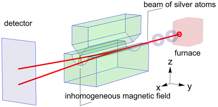
Schematic representation of the Stern–Gerlach experiment.

After this part of the measurement the silver atom in turn interacts with a macrosystem (“detector”) and is finally detected in a rudimentary position measurement. We model this last part of the measurement by an elastic collision of the silver atom with another macroscopic particle P (the “pointer”) with Hilbert space H m = L 2 R 3 , d 3 r 2 . P is initially located at the point (A, 0, C) where the upwards deflected silver atom is expected to arrive at the screen. It must be ensured that the downwardly deflected silver atom does not interact with P. Furthermore, it will be sufficient to simplify the collision as a one-dimensional problem by considering only the coordinate in the direction of the upward deflected beam, which we again denote by x (neglecting the small z component of the beam direction for this part of the calculation).

For future reference, we recall that a Gaussian wave packet satisfying the 1-dimensional free Schrödinger equation can be written in the form

with initial value

Here r _i is one coordinate of the position vector r, m denotes the mass of the particle, v _i a velocity parameter such that mv _i will be the expectation value of r _i -momentum and d will be the standard deviation of the r _i -position observable at t = 0. Generally we have

which describes the well-known spreading of the wave packet with increasing time. This spreading can be neglected for short times, more precisely, for

A general element of the product space H S ⊗ H R = C 2 ⊗ L 2 R 3 , d 3 r 1 can be written in the form of a spinor Ψ ↑ ( r 1 , t ) Ψ ↓ ( r 1 , t ) . We will first concentrate on the first component Ψ_↑(r₁, t). Initially, Ψ_↑(r₁, t = t₁) will be chosen as a Gaussian wave packet at rest. During the first part of the measurement, corresponding to its flight through the magnet, the silver atom will be accelerated into the direction, say, of increasing z₁. The exact calculation of the motion of the silver atom in an inhomogeneous magnetic field would be difficult, but we may assume that, at the end of the first part, at time t₂, the first component Ψ_↑(r₁, t₂) is approximately given by

where we have set r 1 = x 1 , y 1 , z 1 , inserted the mass m₁ of the silver atom into (41) and chosen our space-time coordinate system such that t₂ = 0 and the wave packet has the position expectation value ⟨r₁⟩ = (0, 0, 0) at t = t₂ = 0. The width d₁ > 0 is left unspecified and will be chosen later.

The next part of the measurement is the free time evolution of the silver atom described by ψ_↑(r₁, t) until it collides with the macroscopic particle P at x₁ = A. At time t = t₂ = 0 the macroscopic particle with mass m₂ will be represented by the Gaussian wave packet written in product form

where we have set r 2 = x 2 , y 2 , z 2 and introduced C as the vertical coordinate of the point where the upwards deflected beam hits the screen. The distance A > 0 and the widths d₁, d₂ have to be chosen such that the two wave packets, that of the silver atom and that of the pointer, practically do not overlap at time t = 0.

As noted above, we will simplify the treatment of the collision by considering only the horizontal coordinates x₁ of the silver atom and x₂ of the pointer. Then the collision dynamics is most conveniently calculated by passing to center of mass and relative coordinates

since the motion w.r.t. X will be free if the interaction only depends on x. The inverse transformation is given by

Here we encounter the following problem: If we insert (48) into Ψ_↑(x₁, t)ψ_↑(x₂, t) the result can, in general, not be factored into a wave function depending on X and another one depending on x. This would call our Assumption 1 into question. Fortunately, we can achieve the factorization

for all t by the special choice

as can be shown by a short computation. This condition can be reformulated equivalently by saying that the “dissipation time” t ( i ) = 2 d i 2 m i ℏ , i = 1,2 , of the two wave packets is the same.

The Schrödinger equation describing the collision between the silver atom and the pointer can then be decoupled into two equations of the form

Here M and μ are the total and the reduced mass, resp., defined in the usual way by

and V(x) is the interaction potential. Equation (51) describes a free time evolution for the center of mass wave function Φ_↑(X, t). For the interaction potential we choose a repulsive delta function of the form

which entails that the transmission probability can be neglected and the silver atom will be reflected by the pointer with probability ≈ 1 . Otherwise we would not be able to maintain our Assumption 1. Hence the solution of (52) is practically identical to a perfect reflection at an infinite wall potential and is thus given by a superposition of an incoming wave packet ϕ_↑(x, t) and a reflected one −ϕ_↑(−x, t) for x < 0 and a vanishing wave function for x ≥ 0. At the time t = t₂ = 0 practically only the incoming wave is present and at the time t ≥ t₃ ≔ 2A/v only the reflected wave. This presupposes that the dispersion of the wave packet ϕ_↑(x, t) has not become too large at t = t₃ which will be checked later when concrete number values have been chosen.

We conclude that at time t ≥ t₃ the collision is practically finished and that the total wave function will be of the form

where we have again invoked the condition (50) in order to factorize the result in the specified way.

In order to confirm the Assumption 1 it has to be shown that, for t ≥ t₃, the final pointer state ψ ↑ + ( x 2 , t ) is approximately a coherent state (up to a time-dependent phase factor). To this end we will use the condition (44) for the pointer state which can be translated into θ ≪ 1 if the dimensionless parameter θ is implicitly defined by setting

The details of the calculation will be given in B.

So far we have only considered the first component of the spinor Ψ ↑ ( r 1 , t ) Ψ ↓ ( r 1 , t ) . It would be a straight forward task to repeat the foregoing considerations for the second component by considering the silver atom with spin down being deflected downwards and colliding with a second pointer. But in order to keep the example as simple as possible we do not consider a second pointer and only argue that in this case the silver atom practically will not interact with the first pointer which hence is, for θ ≪ 1, represented by a Gaussian wave packet ψ ↓ + ( r 2 , t ) at rest.

It remains to confirm that, for some time t > t₃ the two pointer states ψ ↑ + ( x 2 , t ) and ψ ↓ + ( x 2 , t ) , which according to B can be approximated by coherent states Ω_↑ and Ω_↓, can be macroscopically distinguished. Recall that Ω_↑ = |x₀, v₀⟩ with x 0 = A m 2 − m 1 m 2 + m 1 + 2 m 1 v m 1 + m 2 t ≈ A + 2 m 1 v m 1 + m 2 t for m₁ ≪ m₂, see (B8), whereas Ω_↓ = |A, 0⟩. Hence the condition of Ω_↑ and Ω_↓ being macroscopically distinct is equivalent to

The consistency of the various assumptions will be examined in the following subsection.

5.2 Choice of concrete values

It is the aim of this subsection to show, by choosing concrete values for the physical quantities of the simplified Stern–Gerlach experiment and for the free parameters α and β of the theory QT*, that the various assumptions we made in the previous subsection are consistent and also in agreement with the general theory of Galilean decoherence that we have developed.

Thus let us assume that a silver atom with mass m₁ = 1.79 × 10⁻²⁵ kg moves with a horizontal velocity of u = 600 m s through a magnet of length L = 0.25 m with an inhomogeneity of ∂ B ∂ z = 120 T m . The time of flight through the magnet is therefore |t₁| = 4.17 × 10⁻⁴ s. The spin 1/2 electron in the outer shell of the silver atom has a magnetic moment of 1 μ B = 9.274 × 1 0 − 24 J T . Due to the vertical acceleration in the inhomogeneous magnetic field, the silver atom finally reaches a vertical velocity of

After leaving the magnet, the silver atom moves horizontally for the time t 3 2 = 3.333 × 1 0 − 4 s until it hits the screen at a horizontal distance of A = 0.2 m.

Next we choose the mass of the macroscopic particle P as m₂ = 10⁸ m₁ = 1.79 × 10⁻¹⁷ kg, approximately corresponding to the mass of a 18 corona viruses. Further let

which, by virtue of (25), (50) and (26), implies

Using these values we will check the consistency of our assumptions. First we estimate the vertical distance Δz = 2C between the two partial beams when they hit the screen as

It can therefore actually be ruled out that the silver atom deflected downwards interacts with the particle P, which is initially located at z 2 = 1 2 Δ z = C .

Next we assume that the duration Δt of the total measuring process will be Δt = 10² τ = 0.5235 s. The times |t₁| and t₃ for the first parts of the measurement can therefore be neglected in comparison with Δt. During the time Δt, the pointer moves by the horizontal distance

This means that the two coherent states Ω_↑ and Ω_↓ can indeed be considered as macroscopically distinct and in this sense the condition (57) can be regarded as fulfilled.

The condition θ ≪ 1 which guarantees that the wave packet of the pointer practically will not spread during the measurement process is satisfied in the sense that

With the shorter collision time t₃ = 6.667 × 10⁻⁴ s the wave packet of the silver atom will not spread either due to (50).

Finally, we consider the decoherence process after the time τ. The width Δη in the Gaussian function (20) assumes the value

Hence the superposition of the two pointer states Ω_↑ and Ω_↓ is damped by a factor which is fapp zero. In contrast, the analogous width Δη₁ for the damping factor of the silver atom, calculated for the whole duration Δt of the measurement, assumes the value

which means that Galilean decoherence of the state of the silver atom can be safely neglected.

To summarize, we can say that a consistent choice of physical quantities is possible for the Stern–Gerlach experiment, which confirms our theory of decoherence by Galilean fluctuations.

References

[1] C. F. von Weizsäcker, Aufbau der Physik, München, Wien, Carl Hanser, 1985.Suche in Google Scholar
[2] J. von Neumann, Matnematische Grundlagen der Quantenmechanik, Berlin, Springer, 1932, (English translation: “Mathematical foundations of quantum mechanics”, Princeton University Press, Princeton, New Jersey, 1955).Suche in Google Scholar
[3] G. Ludwig, Die Grundlagen der Quantenmechanik, Berlin, Springer, 1954.10.1007/978-3-662-37993-6Suche in Google Scholar
[4] G. Ludwig, An Axiomatic Basis for Quantum Mechanics, Volume 2, Quantum Mechanics and Macrosystems, New York, Springer, 1987.10.1007/978-3-642-71897-7Suche in Google Scholar
[5] F. London, E. Bauer, and P. Langevin, La théorie de 1’observation en mécanique quantique, Paris, Hermann, 1939.Suche in Google Scholar
[6] H. EverettIII, ““Relative state” formulation of quantum mechanics,” Rev. Mod. Phys., vol. 29, no. 3, pp. 454–462, 1957. https://doi.org/10.1103/revmodphys.29.454.Suche in Google Scholar
[7] B. S. deWitt, “The Everett-Wheeler interpretation of quantum mechanics,” in Battelle Rencontres, 1967 Lectures in Mathematics and Physics, C. M. deWitt and J. A. Wheeler, Eds., New York, Benjamin, 1968, pp. 318–332.Suche in Google Scholar
[8] D. Bohm and J. Bub, “A proposed solution of the measurement problem in quantum mechanics by a hidden variable theory,” Rev. Mod. Phys., vol. 38, no. 3, pp. 453–469, 1966. https://doi.org/10.1103/revmodphys.38.453.Suche in Google Scholar
[9] R. B. Griffiths, “Consistent histories and the interpretation of quantum mechanics,” J. Stat. Phys., vol. 36, nos. 1–2, pp. 219–272, 1984. https://doi.org/10.1007/bf01015734.Suche in Google Scholar
[10] G. C. Ghirardi, A. Rimini, and T. Weber, “Unified dynamics for microscopic and macroscopic systems,” Phys. Rev. D, vol. 34, no. 2, pp. 470–491, 1986. https://doi.org/10.1103/physrevd.34.470.Suche in Google Scholar PubMed
[11] D. Giulini, E. Joos, C. Kiefer, J. Kupsch, I.-O. Stamatescu, and H. D. Zeh, Eds. Decoherence and the Appearance of a Classical World in Quantum Theory, Berlin, Heidelberg, New York, Springer, 1996.10.1007/978-3-662-03263-3Suche in Google Scholar
[12] R. Penrose, The Emperor’s New Mind: Concerning Computers, Minds and The Laws of Physics, Oxford, UK, Oxford University Press, 1989.10.1093/oso/9780198519737.001.0001Suche in Google Scholar
[13] L. E. Ballentine, “The statistical interpretation of quantum mechanics,” Rev. Mod. Phys., vol. 42, no. 4, pp. 358–381, 1970. https://doi.org/10.1103/revmodphys.42.358.Suche in Google Scholar
[14] L. E. Ballentine, Quantum Mechanics: A Modern Development, 2nd ed. Singapore, World Scientific, 2015.Suche in Google Scholar
[15] G. Ludwig, An Axiomatic Basis for Quantum Mechanics, Volume 1, Derivation of the Hilbert Space Structure, New York, Springer, 1985.10.1007/978-3-642-70029-3_1Suche in Google Scholar
[16] D. Home and M. A. B. Whitaker, “Ensemble interpretations of quantum mechanics. A modern perspective,” Phys. Rep., vol. 210, no. 4, pp. 223–317, 1992. https://doi.org/10.1016/0370-1573(92)90088-h.Suche in Google Scholar
[17] A. Peres, Quantum Theory: Concepts and Methods, Dordrecht, Kluwer, 1993.Suche in Google Scholar
[18] S. Kochen and E. P. Specker, “The problem of hidden variables in quantum mechanics,” J. Math. Mech., vol. 17, no. 1, pp. 59–87, 1967. https://doi.org/10.1512/iumj.1968.17.17004.Suche in Google Scholar
[19] J.-M. Lévy-Leblond, “Galilei group and nonrelativistic quantum mechanics,” J. Math. Phys., vol. 4, no. 6, pp. 776–788, 1963. https://doi.org/10.1063/1.1724319.Suche in Google Scholar
[20] J.-M. Lévy-Leblond, “Nonrelativistic particles and wave equations,” Commun. Math. Phys., vol. 6, pp. 286–311, 1967, https://doi.org/10.1007/bf01646020.Suche in Google Scholar
[21] R. F. Bass, Stochastic Processes, Cambridge Series in Statistical and Probabilistic Mathematis, vol. 33, Cambridge, Cambridge University Press, 2011.Suche in Google Scholar
[22] K. Kraus, States, Effects, and Operations Fundamental Notions of Quantum Theory, Lecture Notes in Physics, vol. 190, Berlin, Springer, 1983.10.1007/3-540-12732-1Suche in Google Scholar
[23] H. J. Lipkin, Quantum Mechanics: New Approaches to Selected Topics, North-Holland, New York, 1973, reprinted by: Courier Corporation, 2014.Suche in Google Scholar
[24] S. Avancini, J. R. Marinelli, and G. Krein, “Compositeness effects in the Bose-Einstein condensation,” J. Phys. A: Math. Gen., vol. 36, no. 34, pp. 9045–9052, 2003. https://doi.org/10.1088/0305-4470/36/34/307.Suche in Google Scholar
[25] P. Céspedes, E. Rufeil-Fiori, P. A. Bouvrie, A. P. Majtey, and C. Cormick, “Description of composite bosons in discrete models,” Phys. Rev. A, vol. 100, no. 1, p. 012309, 2019. https://doi.org/10.1103/physreva.100.012309.Suche in Google Scholar
[26] J. R. Klauder and B. S. Skagerstam, Coherent States: Applications in Physics and Mathematical Physics, Singapore, World Scientific, 1985.10.1142/0096Suche in Google Scholar
[27] E. Scheibe, Die Reduktion physikalischer Theorien, Teil II: Inkommensurabilität und Grenzfallreduktion, Berlin, Springer, 1999.10.1007/978-3-642-59286-7Suche in Google Scholar
[28] P. Strasberg, “Classicality with(out) decoherence: concepts, relation to Markovianity, and a random matrix theory approach,” SciPost Phys., vol. 15, no. 1, p. 024, 2023. https://doi.org/10.21468/scipostphys.15.1.024.Suche in Google Scholar
[29] N. Wiebe and L. E. Ballentine, “Quantum mechanics of hyperion,” Phys. Rev. A, vol. 72, no. 2, p. 022109, 2005. https://doi.org/10.1103/physreva.72.022109.Suche in Google Scholar
[30] M. Schlosshauer, “Classicality, the ensemble interpretation, and decoherence: resolving the hyperion dispute,” Found. Phys., vol. 38, pp. 796–803, 2008, https://doi.org/10.1007/s10701-008-9237-x.Suche in Google Scholar
[31] L. E. Ballentine, “Classicality without decoherence: a reply to Schlosshauer,” Found. Phys., vol. 38, pp. 916–922, 2008, https://doi.org/10.1007/s10701-008-9242-0.Suche in Google Scholar
[32] D. J. Raymond, “How determinate is the “billiard ball universe”,” Am. J. Phys., vol. 35, no. 2, pp. 102–103, 1967. https://doi.org/10.1119/1.1973895.Suche in Google Scholar
[33] L. E. Ballentine, “Quantum-to-classical limit in a Hamiltonian system,” Phys. Rev. A, vol. 70, no. 3, p. 032111, 2004. https://doi.org/10.1103/physreva.70.032111.Suche in Google Scholar
[34] A. S. Holevo, “A note on covariant dynamical semigroups,” Rep. Math. Phys., vol. 32, no. 2, pp. 211–216, 1993. https://doi.org/10.1016/0034-4877(93)90014-6.Suche in Google Scholar
[35] S. Nimmrichter and K. Hornberger, “Macroscopicity of mechanical quantum superposition states,” Phys. Rev. Lett., vol. 110, no. 16, p. 160403, 2013. https://doi.org/10.1103/physrevlett.110.160403.Suche in Google Scholar
[36] B. Schrinski, S. Nimmrichter, B. A. Stickler, and K. Hornberger, “Macroscopicity of quantum mechanical superposition tests via hypothesis falsification,” Phys. Rev. A, vol. 100, no. 3, p. 032111, 2019. https://doi.org/10.1103/physreva.100.032111.Suche in Google Scholar
[37] P. Havas, “Four-dimensional formulations of Newtonian mechanics and their relation to the special and general theory of relativity,” Rev. Mod. Phys., vol. 36, no. 4, pp. 938–965, 1964. https://doi.org/10.1103/revmodphys.36.938.Suche in Google Scholar
[38] C. Brislawn, “Kernels of trace class operators,” Proc. Am. Math. Soc., vol. 104, no. 4, pp. 1181–1190, 1988. https://doi.org/10.2307/2047610.Suche in Google Scholar
© 2025 Walter de Gruyter GmbH, Berlin/Boston
Artikel in diesem Heft
- Frontmatter
- Dynamical Systems & Nonlinear Phenomena
- Controlling the convective heat transfer of shear thinning and shear thickening fluids in parallel plates with magnetic force
- Multistability, chaos and hyperchaos in a novel 3D discrete memristive system: microcontroller implementation and cryptography
- Comparative study of thermally intense cilia and non-cilia generated motion of Ellis’s fluid by using MATHEMATICA 14.1
- Fundamental Concepts of Physical Science
- Nonlinear electrodynamics and its possible connection to relativistic superconductivity: instance of a time-dependent system