Exact solution of the 1D Dirac equation for the inverse-square-root potential 1/x

1 Introduction

Exact solutions of the Dirac equation, which is a relativistic wave equation of fundamental importance in physics [1], are rare. In the one-dimensional case, apart from the piece-wise constant potentials and their generalizations involving the Dirac δ-functions, one may mention the Coulomb, linear, and exponential potentials as follows [2]:

for which, the Dirac equation can be solved in terms of confluent hypergeometric functions, and the potential is given as follows:

for which the Dirac equation can be solved in terms of ordinary hypergeometric functions. Many potentials reported so far, e.g., the Dirac-oscillator [3], [4], Woods-Saxon [5], and Hulthén [6] potentials are particular cases of these four potentials that can be derived by (generally complex) specifications of the involved parameters. Note that the first three potentials given by Equation (1) are particular truncated cases of the classical Kratzer [7], harmonic oscillator [8], and Morse [9] potentials for the Schrödinger equation, while the fourth potential given by Equation (2) in general (if V1V2≠0 and V1≠V2) does not belong to a known Schrödinger potential. However, the solution for this potential can be constructed using the solution of the Schrödinger equation for the Pöschl-Teller potential [10] or that for the Eckart potential [11] (note that the solution for a truncated version of potential (2) with V₂ = 0 can be written using the solution for the Eckart potential).

In the present paper, we introduce a new exactly solvable potential – the inverse-square-root potential – which is given as follows:

A potential of this functional form was applied in the past as a short-range component in phenomenological modeling of the quark-antiquark interaction [12]. The treatment of the potential, however, was so far restricted to the non-relativistic case described by the Schrödinger equation. Here, we show that the time-independent Dirac equation for this potential can be solved exactly. The solution is written in terms of linear combinations of the Hermite functions of a scaled and shifted argument. Based on this exact solution, we find a notable difference as compared to the Schrödinger case. We note that a potential of this functional form appears also in the graphene physics (e.g., the electrostatic potential caused by a gate voltage at the edge of a graphene strip [13]).

We consider the stationary one-dimensional Dirac equation for a spin 1/2 particle of rest mass m and energy E:

with Hamiltonian H=K+П, where K is the kinetic energy operator, and the interaction operator   stands for the potential of the external field. With the general 2 × 2 Hermitian potential matrix given by real functions V, U, W, and S:

where σ0 is the unit matrix and σ1,2,3 are the Pauli matrices. Equation (4) for the two-component spinor wave function ψ=(ψA,ψB)T reads the following equation:

where c is the speed of light and ℏ is the reduced Planck’s constant (we use dimensional variables since this is useful for construction of new solutions using the known ones – see examples below). Without affecting the physical results, one can eliminate U using the phase transformation ψ→e−iφψ with cℏ⋅dφ/dx=U. Hence, we assume U = 0. The resulting system can be solved for several configurations of functions V, W, S of the form a+b/x.

2 Solution for a basic field configuration

A basic field configuration we consider is given as follows:

with arbitrary V_0,1, W₀, S_0,1. Though this potential is defined on the positive semi-axis x > 0, one can extend it to the whole axis x∈(−∞,+∞) by replacing x by |x|. The solution for x < 0 is then readily constructed by replacing x→−x, cℏ→−cℏ in the solution for x > 0.

To solve the Dirac equation for potential (7), we apply the Darboux transformation

to reduce the system to a single second-order differential equation for a new variable w(x). This is achieved by putting the following equations:

where F=1/x. The resulting equation reads as follows:

where the prime denotes differentiation and

In the spin and pseudo-spin symmetry cases, i.e., when S12=V12, the terms proportional to F(x)² and F′(x) vanish, and Equation (12) is reduced to a Schrödinger-like equation for the inverse-square-root potential:

with energy A/(2mc2) and potential −B/(2mc2x).

The general solution of this equation is presented in the study by Ishkhanyan [14]. Rewritten in terms of our parameters, a fundamental solution for real A and B can be presented as follows:

where

and

We note that a second independent fundamental solution can be constructed by the change cℏ→−cℏ in Equations (17) and (18).

Discussing the general case of field configuration (7) for arbitrary parameters, a main result we report is that a fundamental solution of Equation (12) is given as follows:

where

and

We note that, mathematically, this solution applies not only for real parameters but for arbitrary complex parameters V_1,2, W₀, S_1,2, as well as for arbitrary complex variable x. This observation may be useful if one discusses non-Hermitian generalizations of Hamiltonian (5).

This solution is derived by the reduction of Equation (12) to the biconfluent Heun equation [15], [16]:

The solution of which can be expanded in terms of (generally non-integer order) Hermite functions of a scaled and shifted argument [17]:

(see the definition of the non-integer order Hermite function in [18]).

Following the approach of [19], [20], we apply the transformation ψ=φ (z) u(z) with z=2x and φ=eα1z+α2z2 to show that for the field configuration (7), the parameters of the biconfluent Heun equation obey the equations:

(mathematically, this means that the regular singularity of Equation (23) at z = 0 is apparent). With this, the series (24) terminates on the second term thus resulting in a closed-form solution involving just two Hermite functions:

Rewritten in terms of parameters of Equation (12), this yields the solution (19)–(22).

As regards the general solution of Equation (12), it can be written as follows:

with

where c_1,2 are arbitrary constants and ₁F₁ is the Kummer confluent hypergeometric function. We conclude this section by noting that, in general, the involved Hermite and hypergeometric functions are not polynomials because the index ν=γ−α/ε is not an integer.

3 Another field configuration

The solution of the Dirac equation for several other field configurations is constructed in the same way – via reduction to the biconfluent Heun Equation (23). For instance, for the spin symmetric configuration S(x)−V(x)=Cs=constEquation (6) is reduced to the following equations:

For the field configuration

reducing Equation (29) to the biconfluent Heun Equation (23), we verify that the parameters of the resulting equation fulfill Equation (25). As a result, we arrive at a fundamental solution for ψA written as an irreducible linear combination of two Hermite functions:

with

and (compare with (21)–(22))

For completeness, in this case, the general solution of the Dirac equation involving two independent fundamental solutions can be written as follows:

with

where c_1,2 are arbitrary constants.

We note that for the pseudo-spin symmetry configuration S + V = C_p = const with V(x) and W(x) given by Equation (31), a fundamental solution for ψB is constructed by the formal change (ψA,Cs)→(ψB,Cp) and (V1,W1,E)→(−V1,−W1,−E) in Equations (32)–(35).

4 Bound states

To construct bound states, we (i) extend the potential to the whole x-axis x∈(−∞,+∞) by assuming the potential being of argument |x| instead of x, (ii) demand the wave function to vanish at x→±∞, and (iii) demand the wave function to be continuous in the origin x = 0. The solution for x < 0 is readily constructed by noting that the Dirac system (6) for a potential depending on |x| is not changed if one replaces x→−x and cℏ→−cℏ. It then turns out that the continuity condition in the origin results in the equation ψA(0)ψB(0)=0 [21]. This is an important observation stating that for the bound states either the upper component ψA or the lower one ψB should vanish in the origin. As a result, one gets two subsets of eigenvalues – the ones for which ψA(0)=0 and the ones for which ψB(0)=0. We note that the vanishing of the wave function in the origin is a necessary condition for the non-relativistic limit [22].

As an example, consider the following spin symmetric field configuration:

This is a specific configuration that belongs to both families (7) and (31). Both approaches work yielding the same result. If this configuration is viewed as a particular case of the field configuration (7) with V₀ = W₀ = S₀ = 0 and S₁ = V₁, we have

and the general solution of the Dirac Equation (6) for x > 0 is written as follows:

where c_1,2 are arbitrary constants, w is given via parameters A and B by Equations (16)–(18), and w˜ is constructed from w by the change cℏ→−cℏ. As already mentioned above, the solution (ψA−,ψB−) for x < 0 is constructed by the further change x→−x:

The condition of vanishing the wave function at the infinity leads to the simplification c₂ = c₄ = 0 (we note that then ψA,ψA− are real and ψB,ψB− are imaginary if c₁, c₃ are chosen real). With this, the continuity of the wave function at the origin is achieved if

Vanishing of the determinant of this system presents the exact equation for energy spectrum. Since w(−x) = w(x) and w′(−x) = −w′(x), this equation is reduced to w(0)w′(0) = 0 or ψA(0)ψB(0)=0. Thus, for bound states, either ψA or ψB should vanish in the origin.

Consider the case ψA(0). It is readily shown that this condition is rewritten as follows:

This is the exact equation for a subset of energy eigenvalues. We note that this type of spectrum equations that involve two Hermite functions are faced in several other physical situations (see, e.g., [14], [23]). For sgn(AB) = −1, this is exactly the equation encountered when solving the Schrödinger equation for the inverse-square-root potential [14]. It has been shown that the equation possesses a countable infinite set of discrete positive roots ν_n,  n∈ℕ. This set determines the bound-state energy eigenvalues. We note that all ν_n are not integers so that the bound-state wave functions are not polynomials.

The calculation lines are as follows. Substituting Equations (39) into Equation (18), one arrives at the following cubic equation for energy E_n:

The discriminant D=−4c2ℏ2νn2V18(27m2c6ℏ2νn2+V14) of this equation is negative; hence, the cubic has only one real root [16]. This root is conveniently written through the parameter as follows:

The result is the following equation:

Given that ν_n is known via Equation (46), this is an exact expression.

To approximately solve Equation (46), we note that the arguments and indexes of the involved Hermite functions H_ν(z) belong to the left transient layer for which z≈−2ν+1 [24]. Following the approach of [14], we divide Equation (46) by 2νHν−1(−2ν) and apply the proper approximations [24] to show that the equation has solutions only if sgn(AB) = −1. The resulting approximation for the latter case is the following equation:

Here f(ν) is a non-oscillatory function which does not adopt zero, and D₀ is the constant which is given as follows:

This is a highly accurate approximation (see Figure 1).

Figure 1:

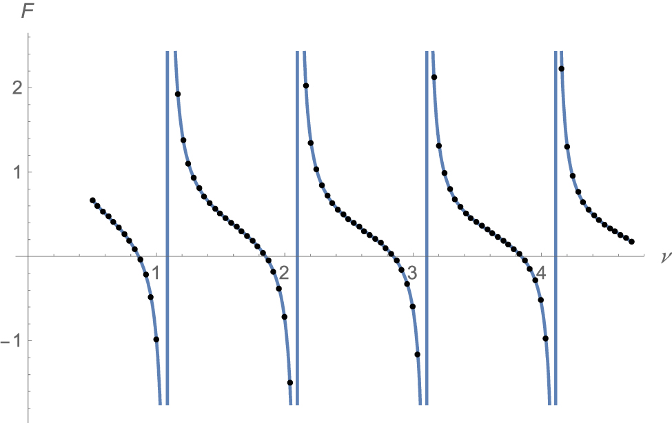
Approximation (50) (filled circles) compared with the exact function F (solid curves). For ν < 1/2 the function does not possess roots.

Thus, the exact Equation (46) is accurately approximated as follows:

Treating the second term of this equation as a perturbation leads to a simple, yet, highly accurate approximation:

The relative error is less than  10⁻⁴ for all orders  n ≥ 2, and the absolute error exceeds  10⁻⁴ only for the first root with  n = 1.

With exact Equation (49), keeping just the first term νn≈n−1/6 in Equation (53), the energy eigenvalues are expanded in terms of n as follows:

This provides a good description of the whole sequence if V12/(mℏc3)≤1 (see Table 1).

Consider now the case ψB(0). It is shown that this condition is rewritten as follows:

which differs from Equation (46) only by the sign of the second term. Acting essentially in the same manner, we find that this equation is well approximated as follows:

with f(ν)=π(2ν)(3ν+1)/6eν/2. Neglecting the second term, we arrive at the following equation:

(note that here  n runs starting from 0). The energy eigenvalues are expanded for large  n as follows:

Starting from  n = 1, this provides a rather good approximation if V12/(mℏc3)≤1 (Table 2).

5 Bound states for the case of electrostatic potential

Consider the following electrostatic potential equation:

For x > 0, this is another particular case of the field configuration (7). Here,

and the general solution of the Dirac Equation (6) is written as follows:

where w_G is the general solution (27), (28) and y, ν, g are given by Equations (20)–(22). After some simplification, we have the following result:

where

The requirement of vanishing of the wave function at x→+∞ gives the following linear relation between c₁ and c₂:

Proceeding in the same manner as in the previous case, we construct the solution of the Dirac Equation (6) for x < 0 by replacing x→−x and cℏ→−cℏ in Equations (20)–(22) and (63)–(65). Note that c₁ and c₂ should be replaced by new arbitrary constants, say, c₃ and c₄, respectively. It is then shown that the requirement of vanishing of the wave function at x→−∞ is satisfied if c₄ = 0. Finally, we verify that the requirement of continuity of the wave function at x = 0 results in the equation ψA(0)ψB(0)=0. Hence, for bound states, either ψA or ψB should vanish in the origin.

Consider the case ψA(0)=0. Since c₄ = 0, it is easier to use the solution for x < 0. Then, after some algebra, the equation ψA(0)=0 is rewritten as (compare with (46) and (55)) follows:

where

This is the exact equation for a subset of the energy spectrum. To treat this equation, we note that, since |E/mc2|<1, the indexes ν, ν−1 and the argument z=−2νE/mc2 of the involved Hermite functions belong to the so called “inner region” for which |z|<2ν. One can then use the standard approximation for the Hermite function for this region [24]:

to arrive at the following highly accurate approximation:

where

The eigenenergies are thus defined as roots of the equation f = k, k∈ℤ.

To get a general insight on the structure of the spectrum, it is useful to examine the behavior of f as a function of energy, the latter being allowed to vary within the interval E∈(−mc2,mc2) (Figure 2). Some characteristics of f are as follows:

where

Figure 2:

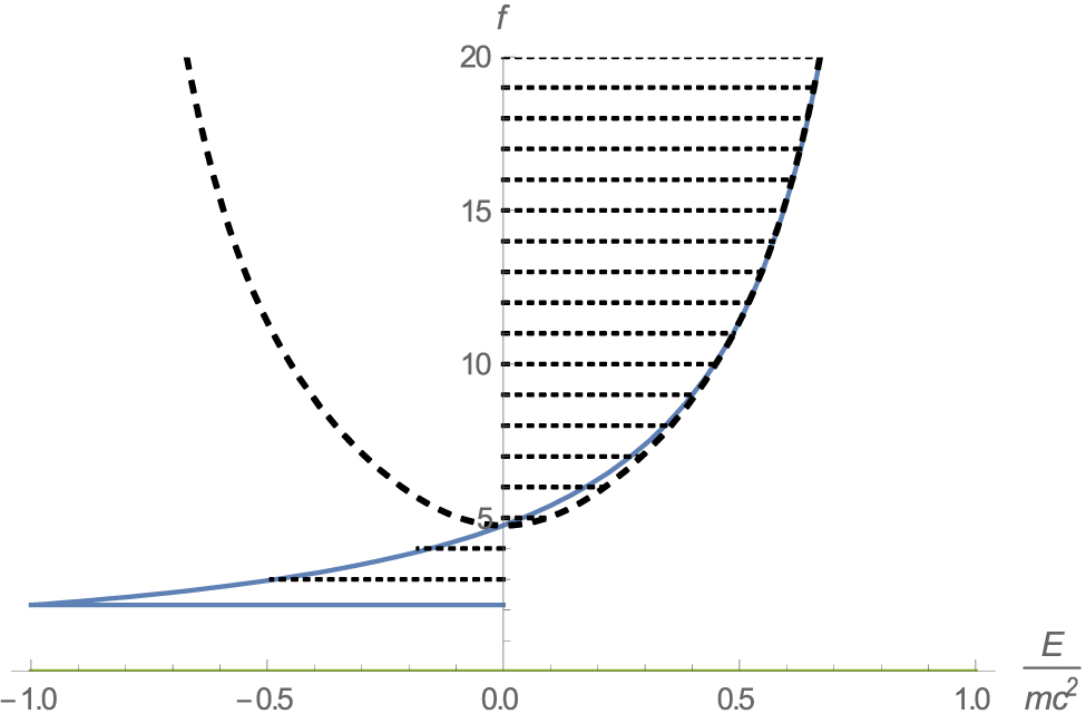
Function f(E) (solid line) for (m,ℏ,c,V1)=(1,1,1,−3). The intersections of horizontal dotted lines with f(E) give the positions of energy levels E_n. There are only two negative eigenenergies for given parameters. The dashed line shows approximation (78).

The function starts from the minimal value f_min at E = −mc², adopts f₀ at E = 0, and diverges to plus infinity at E→+mc2. Since the function has a restricted variation range on the negative interval E∈(−mc2,0), it is understood that there exists only a finite number of negative eigenenergies while the number of positive eigenenergies is infinite. The number of negative eigenenergies is exactly given as follows:

where ⌊…⌋ denotes the floor of a number.

For negative energies E < 0, the function f(E) is well approximated by the parabola

while an appropriate approximation for positive energies E > 0 is

with

Note that a is a small number: a≈−0.07.

With these approximations, one arrives at the following approximate spectrum. If the energy levels are numbered by a positive integer n running from one to infinity, for negative energy levels E_n < 0 we have the following equation:

where n runs from one to n₋. For positive energy levels E_n > 0, using Equation (68), we have the following equation:

where n runs from n₋ + 1 to infinity. This is a rather accurate result for all orders n and for any V₁. Starting from a few lowest energy levels, the relative error is of the order or less than 10⁻³. The comparison of approximation (80) with the exact result for V12/(mℏc3)=1 is shown in Table 3.

We note that for large n→∞, the spectrum behaves as follows:

This result, which is asymptotically exact, indicates that the Maslov index μ=−{f∞} (fractional part of the correction to n [25], [26]) depends on the potential’s strength V₁. This is a notable feature that differs the Dirac case from the Schrödinger one. We recall that in the Schrödinger case, the Maslov index is μ=−1/6 [14].

The bound states corresponding to the case when the upper component of the wave function is even and the lower component is odd, that is, when ψB(0)=0, are treated in the same manner. The exact equation for the second subset of the energy spectrum corresponding to this case is reduced to the following eqaution:

which differs from Equation (67) only by the sign of the second term. An accurate approximation of this equation reads the following equation:

with

which differs from Equation (71) only by the sign of 1/4. Doing the same steps as in the previous case, we arrive at the approximate spectrum given by the same Equations (80)–(82) with f_min, f₀, f_∞ modified such as 1/4 is replaced by −1/4. The two subsets of energy levels for V12/(mℏc3)=1 corresponding to the cases ψA(0)=0 and ψB(0)=0 are compared in Table 4. As seen, the second subset possesses an additional negative level E≈−0.965886, the other levels being located between two adjacent levels of the first subset.

References

[1] W. Greiner, Relativistic Quantum Mechanics. Wave equations, Berlin, Springer, 2000.10.1007/978-3-662-04275-5Suche in Google Scholar
[2] V. G. Bagrov and D. M. Gitman, The Dirac Equation and its Solutions, Boston, De Gruyter, 2014.10.1515/9783110263299Suche in Google Scholar
[3] P. A. Cook, “Relativistic harmonic oscillators with intrinsic spin structure,” Lett. Nuovo Cimento, vol. 1, pp. 419–426, 1971, https://doi.org/10.1007/bf02785170.Suche in Google Scholar
[4] M. Moshinsky and A. Szczepaniak, “The Dirac oscillator,” J. Phys. A, vol. 22, pp. L817–L819, 1989, https://doi.org/10.1088/0305-4470/22/17/002.Suche in Google Scholar
[5] P. Kennedy, “The Woods–Saxon potential in the Dirac equation,” J. Phys. A, vol. 35, pp. 689–698, 2002, https://doi.org/10.1088/0305-4470/35/3/314.Suche in Google Scholar
[6] J. Y. Guo, Y. Yu and S. W. Jin, ”Transmission resonance for a Dirac particle in a one-dimensional Hulthén potential” Cent. Eur. J. Phys., vol. 7, pp. 168–174, 2009. https://doi.org/10.2478/s11534-008-0127-9.Suche in Google Scholar
[7] A. Kratzer, “Die ultraroten Rotationsspektren der Halogenwasserstoffe,” Z. Phys., vol. 3, pp. 289–307, 1920, https://doi.org/10.1007/bf01327754.Suche in Google Scholar
[8] E. Schrödinger, “Quantisierung als Eigenwertproblem,” Ann. Phys., vol. 76, pp. 361–376, 1926, https://doi.org/10.1002/andp.19263840602.Suche in Google Scholar
[9] P. M. Morse, “Diatomic molecules according to the wave mechanics. II. Vibrational levels,” Phys. Rev., vol. 34, pp. 57–64, 1929, https://doi.org/10.1103/physrev.34.57.Suche in Google Scholar
[10] G. Pöschl and E. Teller, “Bemerkungen zur Quantenmechanik des anharmonischen Oszillators,” Z. Phys., vol. 83, pp. 143–151, 1933, https://doi.org/10.1007/bf01331132.Suche in Google Scholar
[11] C. Eckart, “The penetration of a potential barrier by electrons,” Phys. Rev., vol. 35, pp. 1303–1309, 1930, https://doi.org/10.1103/physrev.35.1303.Suche in Google Scholar
[12] X. Song, H. Lin, “A new phenomenological potential for heavy quarkonium,” Z. Phys. C. Particles Fields, vol. 34, pp. 223–231, 1987. https://doi.org/10.1007/BF01566763.Suche in Google Scholar
[13] P. G. Silvestrov and K. B. Efetov, “Charge accumulation at the boundaries of a graphene strip induced by a gate voltage: Electrostatic approach,” Phys. Rev. B, vol. 77, p. 155436, 2008, https://doi.org/10.1103/physrevb.77.155436.Suche in Google Scholar
[14] A. M. Ishkhanyan, “Exact solution of the Schrödinger equation for the inverse square root potential,” Eur. Phys. Lett., vol. 112, p. 10006, 2015, https://doi.org/10.1209/0295-5075/112/10006.Suche in Google Scholar
[15] A. Ronveaux, Ed. Heun’s Differential Equations, London, Oxford Univ. Press, 1995.10.1093/oso/9780198596950.001.0001Suche in Google Scholar
[16] NIST Handbook of Mathematical Functions, New York, Cambridge Univ. Press, 2010.Suche in Google Scholar
[17] T. A. Ishkhanyan and A. M. Ishkhanyan, “Solutions of the bi-confluent Heun equation in terms of the Hermite functions,” Ann. Phys., vol. 383, pp. 79–91, 2017, https://doi.org/10.1016/j.aop.2017.04.015.Suche in Google Scholar
[18] N. N. Lebedev and R. R. Silverman, Special Functions and their Applications, New York, Dover Publications, 1972.Suche in Google Scholar
[19] A. Ishkhanyan and V. Krainov, “Discretization of Natanzon potentials,” Eur. Phys. J. Plus, vol. 131, p. 342, 2016, https://doi.org/10.1140/epjp/i2016-16342-9.Suche in Google Scholar
[20] A. M. Ishkhanyan, “Schrödinger potentials solvable in terms of the general Heun functions,” Ann. Phys., vol. 388, pp. 456–471, 2018. https://doi.org/10.1016/j.aop.2017.11.033.Suche in Google Scholar
[21] R. L. Hall and P. Zorin, “Nodal theorems for the Dirac equation in d ≥ 1 dimensions,” Ann. Phys. (Berlin), vol. 526, pp. 79–86, 2014. https://doi.org/10.1002/andp.201300161.Suche in Google Scholar
[22] M. Znojil, “Comment on Conditionally exactly soluble class of quantum potentials,” Phys. Rev. A, vol. 61, p. 066101, 2000. https://doi.org/10.1103/PhysRevA.61.066101.Suche in Google Scholar
[23] A. S. de Castro, “Comment on Fun and frustration with quarkonium in a 1 + 1 dimension,” Am. J. Phys., vol. 70, pp. 450–451, 2002. https://doi.org/10.1119/1.1445407.Suche in Google Scholar
[24] G. Szegö, Orthogonal Polynomials, 4th ed. Providence, American Mathematical Society, 1975.Suche in Google Scholar
[25] A. M. Ishkhanyan and V. P. Krainov, “Maslov index for power-law potentials,” JETP Lett., vol. 105, pp. 43–46, 2017. https://doi.org/10.1134/S0021364017010106.Suche in Google Scholar
[26] C. Quigg and J. L. Rosner, “Quantum mechanics with applications to quarkonium,” Phys. Rep., vol. 56, pp. 167–235, 1979, https://doi.org/10.1016/0370-1573(79)90095-4.Suche in Google Scholar
© 2020 Walter de Gruyter GmbH, Berlin/Boston
Artikel in diesem Heft
- Frontmatter
- Atomic, molecular & chemical physics
- Systematic calculations of energy levels and transitions rates in Mo XXVIII
- Dynamical systems & nonlinear phenomena
- Gap solitons supported by an optical lattice in biased photorefractive crystals having both the linear and quadratic electro-optic effect
- Hydrodynamics
- Permanent solutions for some oscillatory motions of fluids with power-law dependence of viscosity on the pressure and shear stress on the boundary
- Quantum Theory