Riemann–Hilbert Problem and Multi-Soliton Solutions of the Integrable Spin-1 Gross–Pitaevskii Equations

1 Introduction

The nonlinear Schrödinger (NLS) equation and its variants are well known as general models for solitons and nonlinear waves, as well as relevant phenomenology, in many areas of physics containing water waves, plasmas, Bose-Einstein condensates (BECs), nonlinear optics, etc. [1], [2], [3], [4], [5], [6], [7], [8], [9], [10], [11]. Among different solutions of these equations, the soliton in some related fields has begun to attract attention in recent years. In 1967s, based on the original inverse scattering transformation (IST) [12], [13], [14], an effective and convenient way [i.e. Riemann–Hilbert (RH) method] is first proposed by Novikov and coworkers [15] to construct soliton solutions of nonlinear equations in their article. Very recently, Yang, Wang, Geng, Guo, etc. [16], [17], [18], [19], [20], [21], [22], [23], [24], [25], [26], [27], [28], [29], [30], [31] have made a great contribution in this field.

It is well known that the coupled Gross–Pitaevskii equation is often used to describe the interactions among the modes in nonlinear optics, components in BECs, etc. Therefore, in this article, we mainly focus on the integrable spin-1 Gross–Pitaevskii (SGP) equation [32], [33], [34]:

where q−1=q−1(x,t), q0=q0(x,t), q1=q1(x,t) are the sufficiently smooth functions. The four types of parameters: (a,b)=[(1,1),(1,−1),(−1,1),(−1,−1)] in the SGP system (1) correspond to the four roles of the self-cross-phase modulation (nonlinearity) and spin-exchange modulation, respectively, that is, (attractive, attractive), (attractive, repulsive), (repulsive, attractive), and (repulsive, repulsive). Equation (1) is still integrable. Its Lax pair reads

where Ψ=Ψ(x,t,λ) is a column vector function of the spectral parameter λ, and

where

In what follows, we let a = b = 1 for the convenience of the analysis.

Recently, there are many investigations on solutions of integrable SGP system (1) [35], [36], [37], [38], [39], [40]. For example, in [32], Fokas method is used to investigate the initial-boundary value problem for the integrable SGP (1). In addition, a similarity transformation is used to investigate its non-autonomous multi-rogue wave solutions [34]. It is well known that RH method is a powerful and effective approach to derive multi-soliton solutions. However, as (1) involves a 4 × 4 matrix spectral problem, the RH problem (RHP) for (1) is rather complicated to study. The research in this direction, to the best of the authors’ knowledge, has not been investigated before. The principal aim of the present article is to investigate N-soliton solutions of (1) by utilizing RH method. Besides, we also make some graphical analysis of these solutions.

The structure of this article is given as follows. In the following section, starting from the Lax pair we construct the RHP of (1). In Section 3, we derive N-soliton solutions of (1). Finally, some conclusions and discussions are provided in Section 4.

2 Riemann–Hilbert Problem

In the present section, we consider the inverse scattering transform (IST) for (1) using the RH formulation.

For the sake of convenience, a new matrix spectral function J=J(x,t,λ) is defined by the transform:

such that the Lax pair (2) can be transformed into another equivalent form:

where

and [Λ,J]=ΛJ−JΛ is the commutator. In addition, the two matrix Q and Q~ is traceless. For the sake of convenience, we notice that there is a symmetry relation for Q in (5a):

where † means the Hermitian of a matrix.

For the scattering problem, let us first introduce matrix Jost solutions J±(x,λ) with the following asymptotic condition:

Here 𝕀 is a 4 × 4 identity matrix, and the subscripts of J denote which end of the x axis the boundary conditions are taken. Then, according to tr(Q) = 0 and Abel’s formula, we obtain det(J±)=1 for all x. In the following, we denote E=eiλΛx. As Ψ=J+E and Φ=J−E are both solutions of (5a), they can be related by a scattering matrix:

where

is a scattering matrix. Due to det(J±)=1, we have det(S(λ))=1. Besides, (Φ^,Ψ^) meets the first spectral equation in (5a), i.e.

If we treat the QΨ term in (11) as a inhomogeneous term and note that the solution to the (11) on its left hand is E, then the Jost solutions J_± can be explicitly obtained by the Volterra integral equations

Therefore, J_± allows analytical continuations off the axis λ∈ℝ when the integrals on their right-hand sides converge. It is not hard to check that ([J+]1,[J+]2,[J+]3,[J−]4) allow analytic extensions to upper half λ-plane ℂ⁺. In addition, ([J−]1,[J−]2,[J−]3,[J+]4) can be analytically extendible to the lower half λ-plane ℂ⁻. If we express (Φ^,Ψ^) as a collection of columus:

then the Jost solutions

and (ϕ1,ϕ2,ϕ3,ψ4)eiλΛx are analytic for λ∈ℂ+, λ∈ℂ−, respectively. In addition, from the equations (12), we see that

In what follows, we must construct the analytic counterpart of P⁺ in ℂ⁻. To this end, we should consider adjoint equation of (5a):

It is easy to find the matrix inverses of J_± admit the adjoint (10). Let us introduce

Then by similar techniques as used above, we can obtain that adjoint Jost solutions

are analytic in λ∈ℂ−. In a similar way, we can also find that

To sum up, we have obtained two matrix functions P₁ and P₂, which are analytic for ℂ⁺ and ℂ⁻, respectively. Hence, we obtain an RHP for the GSP system (1)

where

and the canonical normalization condition for the RHP (20) is

The solution to the RHP (20) will not be unique if the zeros of det(P+) and det(P−) in the upper and lower half of the λ plane are not also specified, and the kernel structures of P^± at these zeros are not provided. To this end, we suppose that the RHP (20) is irregular. Here, the irregularity denotes both detP1 and detP2 have certain zeros in their analytic domains. In view of the definitions of P^± and scattering relations between J⁺ and J⁻, we can find det(P+)=s44 and det(P−)=s^44. Assume that s₄₄ admits zeros {λk∈ℂ+,1≤k≤N} and s^44 admits zeros {λk∈ℂ−,1≤k≤N}. For convenience, we suppose that all zeros {(λk,λ^k),k=1,2,⋯,N} are simple zeros of (s44,s^44), which is a general case. Here, v_k and v^k(1≤k≤N) are nonzero column and vectors, respectively, satisfying

In what follows, we construct the IST of the GSP system (1), from which we recover q−1,q0,q1 by using the scattering data. Thus, we expand P⁺ as

then putting it into (5a), and comparing O(1) terms yields

which means that q−1, q₀, q₁ can be obtained as

where P1+=(Pij)4×4.

The symmetry relation (7) of the matrix Q leads to symmetry properties in the scattering matrix and the Jost functions. Thus from (5a), we obtain

Using the large-x boundary conditions of J_± and (16), we know that

In view of this property (28) as well as definitions (14) and (18), we can find that the analytic solution P^± meets the involution property

In view of the relation (9), we find that S admits the following involution property

From the above involution property, we have the symmetry relation λ^k=λk∗ for the whole zeros of s₄₄ and s^44. In order to get the symmetry relations for the eigenvectors v_k and v^k, we use the Hermitian of the first equation in (23). Therefore, from (29), we get

By comparing it with second equation in (23), one can obtain vk†=v^k.

In order to construct the spatial evolutions for vectors v_k(x, t), using the x derivative to P+(λk,x)vk and (5a), we have

i.e.

In the same way, the time dependence on P+(λk,x)vk can be obtained as follows:

i.e.

Then by combining these results, one can obtain

in which (vk0,v^k0) are now constant vectors.

In the following section, the above results will be applied to construct the multi-soliton solutions of the GSP (1).

3 Multi-Soliton Solutions

In this section, the multi-soliton solutions to (1) will be constructed by using the RHP (20) with G=𝕀. The solutions to the RHP have been presented in [41], [42] and the conclusions is

where the matrix M is defined by

Then utilizing (36) and (37), from (26) we can obtain the multi-soliton solutions for (1):

Figure 1:

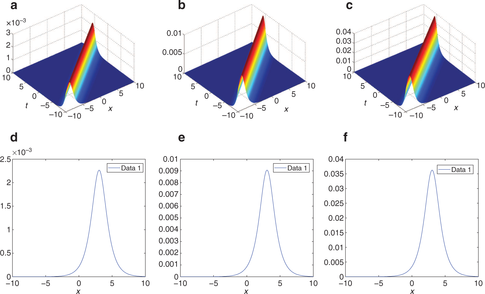
(Colour online) The single soliton via solutions (44) (|q−1|2, |q0|2, |q1|2) with parameters: α1=1,β1=2,γ1=4,λ1=0.3+0.5i. (a)–(c) Perspective view of the real part of the wave. (d)–(f) The wave propagation pattern of the wave along the x axis.

Through above analysis, the multi-soliton solutions for the GSP (1) can be written out explicitly as

with

where θk=iλkx+2iλk2t, and we have taken vk0=(αk,βk,γk,1) without loss of generality. In what follows, we will consider the dynamics of the one-soliton solution and two-soliton solution to the integrable GSP system (1).

3.2 Two-Soliton Solution

In a similar way, taking N = 2 in (40) with (41), (40) can be reduced to a two-soliton solution of the GSP system (1):

(47){q−1(x,t)=2iα1e(θ1∗−θ1)(M−1)11+2iα1e(θ2∗−θ1)(M−1)12+2iα2e(θ1∗−θ21)(M−1)21+2iα2e(θ2∗−θ2)(M−1)22q0(x,t)=2iβ1e(θ1∗−θ1)(M−1)11+2iβ1e(θ2∗−θ1)(M−1)12+2iβ2e(θ1∗−θ2)(M−1)21+2iβ2e(θ2∗−θ2)(M−1)22q1(x,t)=2iγ1e(θ1∗−θ1)(M−1)11+2iγ1e(θ2∗−θ1)(M−1)12+2iγ2e(θ1∗−θ1)(M−1)21+2iγ2e(θ2∗−θ2)(M−1)22

Figure 2:

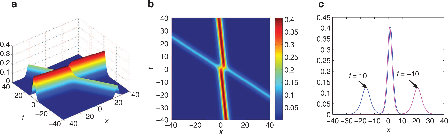
(Colour online) The two-bell soliton solution via (47) (|q−1|2) with parameters: α1=1, α2=i, β1=1+i, β2=0.5i, γ1=2+2i, γ2=i, λ1=0.3i, λ2=0.5i. (a) Perspective view of the real part of the wave. (b) The overhead view of the wave. (c) The wave propagation pattern of the wave along the x axis.

Figure 3:

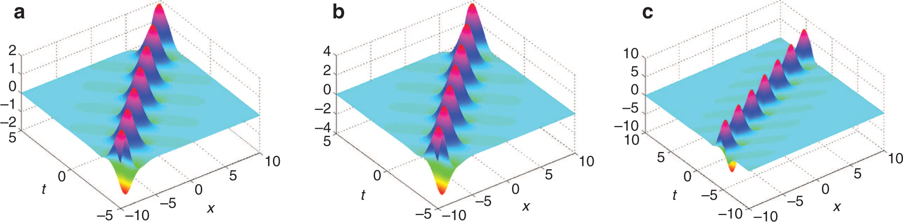
(Colour online) The breather-type solution via (47) (|q−1|2, |q0|2, |q1|2) with parameters: α1=1+1.4i, α2=1.4−1.2i, β2=2+3i, β1=2, γ1=4+3i, γ2=0.5+0.6i, λ1=0.5+0.6i, λ2=−0.3+0.9i. (a)–(c) Perspective view of the real part of the wave.

where M=(mkj)2×2 with

{m11=(|α1|2+|β1|2+|γ1|2)exp(θ1+θ1∗)+exp(−θ1−θ1∗)λ1∗−λ1,m12=(α1∗α2+β1∗β2+γ1∗γ2)exp(θ1∗+θ2)+exp(−θ1∗−θ2)λ1∗−λ2,m21=(α1α2∗+β1β2∗+γ1γ2∗)exp(θ1+θ2∗)+exp(−θ1−θ2∗)λ2∗−λ1,m22=(|α2|2+|β2|2+|γ2|2)exp(θ2+θ2∗)+exp(−θ2−θ2∗)λ2∗−λ2,

and θm=iλmx+2iλm2t(m=1,2). The two-bell soliton interactions governed by the above equation are shown in Figure 2. As shown in Figure 3, we can see that the three constituent solitons have equal velocity; thus, they stay together to form a bound soliton in each component, which moves at the same speed. In addition, we find that the width of the soliton solution changes periodically with time and thus can reveal the usual breather wave features; this solution is called “breather soliton.”

4 Conclusions and Discussions

In this work, the integrable SGP (1) has been systematically discussed by employing RH method. Then N-soliton solutions of (1) are obtained by using its RH formulation. In order to help the readers understand the soliton solutions better, we have made some graphical analysis of those solutions. Our results can be used to further enrich the dynamic behavior of the nonlinear wave fields. The article shows that the effective method (i.e. RH method) provides a direct and powerful mathematical tool to seek new exact solutions of nonlinear evolution equations (NLEEs), which should be suitable to study other models in mathematical physics and engineering. Comparing with the soliton solution formulae obtained here and those constructed by Darboux transformation and Hirota bilinear method, it is very clear that the expressions are much simpler. More importantly, as the coupled NLS equations arise in a wide variety of physical subjects such as nonlinear optics, water waves, BECs, etc, these results should prove helpful to the studies of those physical problems.

References

[1] M. J. Ablowitz and P. A. Clarkson, Solitons, Nonlinear Evolution Equations and Inverse Scattering, Cambridge University Press, Cambridge, UK 1990.10.1017/CBO9780511623998Search in Google Scholar
[2] G. P. Agrawal, Nonlinear Fiber Optics, Academic Press, San Diego 1995.Search in Google Scholar
[3] L. Pitaevskii and S. Stringari, Bose-Einstein Condensation, Oxford University Press, Oxford 2003.Search in Google Scholar
[4] R. Carretero-González, D. J. Frantzeskakis, and P. G. Kevrekidis, Nonlinearity 21, R139 (2008).10.1088/0951-7715/21/7/R01Search in Google Scholar
[5] Y. Wang, Y. Yang, S. He, W. Wang, AIP Adv. 7, 105209 (2017).10.1063/1.5001157Search in Google Scholar
[6] Y. V. Kartashov, B. A. Malomed, and L. Torner, Rev. Mod. Phys. 83, 247 (2011).10.1103/RevModPhys.83.247Search in Google Scholar
[7] V. E. Zakharov, J. Appl. Mech. Tech. Phys. 9, 190 (1968).10.1007/BF00913182Search in Google Scholar
[8] A. Hasegawa and F. Tappert, Appl. Phys. Lett. 23, 142 (1973).10.1063/1.1654836Search in Google Scholar
[9] D. J. Benney and A. C. Newell, Stud. Appl. Math. 46, 133 (1967).10.1002/sapm1967461133Search in Google Scholar
[10] G. P. Agrawal, Nonlinear Fiber Optics, Academic Press, San Diego 2001.Search in Google Scholar
[11] S. V. Manakov, Sov. Phys. JETP 38, 248 (1974).Search in Google Scholar
[12] M. J. Ablowitz and P. Clarkson, Soliton, Nonlinear Evolution Equations and Inverse Scattering, Cambridge University Press, Cambridge, UK 1991.10.1017/CBO9780511623998Search in Google Scholar
[13] M. J. Ablowitz, D. J. Kaup, A. C. Newell, and H. Segur, Stud. Appl. Math. 53, 249 (1974).10.1002/sapm1974534249Search in Google Scholar
[14] C. S. Gardner, J. M. Greene, M. D. Kruskal, and R. M. Miura, Phys. Rev. Lett. 19, 1095 (1967).10.1103/PhysRevLett.19.1095Search in Google Scholar
[15] S. Novikov, S. Manakov, L. Pitaevskii, and V. Zakharov, Theory of Solitons: The Inverse Scattering Method, Consultants Bureau, New York and London 1984.Search in Google Scholar
[16] M. J. Ablowitz and A. S. Fokas, Complex Variables: Introduction and Applications, Cambridge University Press, Cambridge, UK 2003.10.1017/CBO9780511791246Search in Google Scholar
[17] A. S. Fokas, A Unified Approach to Boundary Value Problems, in CBMS-NSF Regional Conference Series in Applied Mathematics, SIAM 2008.10.1137/1.9780898717068Search in Google Scholar
[18] X. Geng and J. Wu, Wave Motion 60, 62 (2016).10.1016/j.wavemoti.2015.09.003Search in Google Scholar
[19] B. Guo and L. Ling, J. Math. Phys. 53, 133 (2012).10.1063/1.4732464Search in Google Scholar
[20] D. S. Wang, D. J. Zhang, and J. Yang, J. Math. Phys. 51, 023510 (2010).10.1063/1.3290736Search in Google Scholar
[21] J. Xu and E. G. Fan, Proc. R. Soc. Lond. A 469, 20130068 (2013).10.1098/rspa.2013.0068Search in Google Scholar PubMed PubMed Central
[22] J. Xu, E.G. Fan, and Y. Chen, Math. Phys. Anal. Geom. 16, 253 (2013).10.1007/s11040-013-9132-3Search in Google Scholar
[23] W. X. Ma, J. Geom. Phys. 132, 45 (2018).10.1016/j.geomphys.2018.05.024Search in Google Scholar
[24] D. Kaup and J. Yang, Inverse Probl. 25, 105010 (2009).10.1088/0266-5611/25/10/105010Search in Google Scholar
[25] J. Yang, Nonlinear Waves in Integrable and Nonintegrable Systems, SIAM 2010.10.1137/1.9780898719680Search in Google Scholar
[26] J. Yang and D. Kaup, J. Math. Phys. 50, 121 (2009).10.1063/1.3075567Search in Google Scholar
[27] Y. S. Zhang, Y. Cheng, and J. S. He, J. Nonlinear Math. Phys. 24, 210 (2017).10.1080/14029251.2017.1313475Search in Google Scholar
[28] S. F. Tian. J. Differ. Equ. 262, 506 (2017).10.1016/j.jde.2016.09.033Search in Google Scholar
[29] S. F. Tian, J. Phys. A: Math. Theor. 50, 395204 (2017).10.1088/1751-8121/aa825bSearch in Google Scholar
[30] S. F. Tian, Proc. R. Soc. Lond. A 472, 20160588 (2016).10.1098/rspa.2016.0588Search in Google Scholar PubMed PubMed Central
[31] Y. Xiao and E. G. Fan, Chin. Ann. Math. Ser. B 37, 373 (2016).10.1007/s11401-016-0966-4Search in Google Scholar
[32] Z. Y. Yan, Chaos 27, 053117 (2017).10.1063/1.4984025Search in Google Scholar PubMed
[33] Y. Wang, Y. Zhou, S. Zhou, and Y. Zhang, Phys. Rev. E 94, 012225 (2016).10.1103/PhysRevE.94.012225Search in Google Scholar PubMed
[34] L. Li and F. J. Yu, Sci. Rep. 7, 10638 (2017).10.1038/s41598-017-10205-4Search in Google Scholar PubMed PubMed Central
[35] J. Ieda, T. Miyakawa, and M. Wadati, Phys. Rev. Lett. 93, 194102 (2004).10.1103/PhysRevLett.93.194102Search in Google Scholar PubMed
[36] Y. Kawaguchi and M. Ueda, Phys. Rep. 520, 253 (2012).10.1016/j.physrep.2012.07.005Search in Google Scholar
[37] M. Olshanii, Phys. Rev. Lett. 81, 437 (1998).10.1103/PhysRevLett.81.437Search in Google Scholar
[38] G. P. Agrawal, Nonlinear Fiber Optics, 4th ed., Academic Press, San Diego, CA 2006.10.1016/B978-012369516-1/50011-XSearch in Google Scholar
[39] J. Ieda, T. Miyakawa, and M. Wadati, J. Phys. Soc. Jpn. 73, 2996 (2004).10.1143/JPSJ.73.2996Search in Google Scholar
[40] L. Li, Z. Li, B. A. Malomed, D. Mihalache, and W. M. Liu, Phys. Rev. A 72, 033611 (2005).10.1103/PhysRevA.72.033611Search in Google Scholar
[41] V. E. Zakharov, S. V. Manakov, S. P. Novikov, and L. P. Pitaevskii, The Theory of Solitons: The Inverse Scattering Method, Consultants Bureau, New York 1984.Search in Google Scholar
[42] J. Yang, Nonlinear Waves in Integrable and Non-Integrable Systems, Society for Industrial and Applied Mathematics 2010.10.1137/1.9780898719680Search in Google Scholar
©2018 Walter de Gruyter GmbH, Berlin/Boston
Articles in the same Issue
- Frontmatter
- General
- Einstein’s “Clock Hypothesis” and Mössbauer Experiments in a Rotating System
- Atomic, Molecular & Chemical Physics
- Dual Fabry–Pérot Interferometric Carbon Monoxide Sensor Based on the PANI/Co3O4 Sensitive Membrane-Coated Fibre Tip
- Study of the Geometric Structures, Electronic and Magnetic Properties of Aluminium-Antimony Alloy Clusters
- A Density Functional Theory Study on the Structures and Electronic Properties of XAln (X = Br, I; n = 3–15) Clusters
- Dynamical Systems & Nonlinear Phenomena
- Three-Dimensional Instability of Opposite Polarity Nonthermal Dusty Plasma