1 Introduction
I. We study the equilibrium equations for a plasma with zero electrical resistance [1], [2], [3]:
(1)J×B=gradp,curlB=μJ,divB=0,
where B is the magnetic field, J – the electric current, μ – the magnetic permeability, p – the pressure. In papers [4] and [5], Taylor asserted that at the non-zero plasma viscosity the magnetohydrodynamic turbulence leads to the plasma relaxation towards a final state where magnetic field B(x) satisfies the Beltrami equation
(2)curlB(x)=αB(x)
with a constant α, and has the same integral of helicity [6] as the original plasma configuration.
As known [7], [8], in the ideal magnetohydrodynamics with vanishing electrical resistance the magnetic field B(t,x) is transformed in time by the plasma flow diffeomorphisms (or “is frozen in the flow”). Therefore, the closed magnetic field lines are transformed in time into the isotopically equivalent closed magnetic lines.
II. In the 1958 paper [1], Kruskal and Kulsrud proved for the plasma equilibrium (1) that a surface p(x)=const that “lies in a bounded domain and has no edges” in the general case is “a topological torus” that is “made up of lines of magnetic forceB(x)” and stated that “under normal circumstances each surface p = P(excepting a set of values of P of measure zero) is traversed ergodically and consequently determined by any line of force contained in it.”
In the 1959 paper [9], Newcomb stated “It is easy to verify that the lines of force on a pressure surface are closed if and only ifι(P)/2πis rational; if it is irrational, the lines of force cover the surface ergodically.” Here ι(P) is the rotational transform connected with the safety factor q(P) [10] by the relation q(P)=2π/ι(P) [11], [12].
A study of safety factor q for concrete plasma equilibria may prove to be important for the problem of controlled fusion because the stability properties of a toroidal plasma equilibrium are connected with its q profile [13].
Safety factor for the time-dependent axisymmetric magnetic fields is studied in [14].
III. Axisymmetric steady magnetic fields have the form
(3)B(r,z)=−1r∂ψ∂ze^r+1r∂ψ∂re^z+w(r,z)re^φ,
where ψ(r,z) is a flux function, 2πw(r,z) is the magnetic flux circulation (analog of the swirl in fluid dynamics) and e^r, e^z, e^φ are vectors of unit length along the axes of the cylindrical coordinates r, z, φ. The steady axisymmetric (1) were reduced in [2], [3] to the nonlinear Grad–Shafranov equation
(4)ψrr−1rψr+ψzz=r2dFdψ−𝒢d𝒢dψ,
where F(ψ) and 𝒢(ψ) are arbitrary smooth functions of ψ connected with the pressure p and the circulation 2πw(r,z) by the relations
(5)F(ψ)=−μp(r,z),𝒢(ψ)=w(r,z).
In Section 2 we study the general Grad–Shafranov equation (4) and derive an exact formula for the limit of the safety factor q at a magnetic axis for all solutions to (4). The derived formula yields that the limit value qm of the safety factor at a magnetic axis is finite and non-zero.
IV. There are three cases for that (4) becomes linear:
(6)F(ψ)=λψ+C,𝒢(ψ)=αψ,
(7)F(ψ)=c2ψ2+C,𝒢(ψ)=αψ,
(8)F(ψ)=λψ+C,𝒢(ψ)=α22ψ−ψ0,
where α,λ,C,ψ0 are arbitrary constants. Exact solutions for the case (7) that are global plasma equilibria modeling astrophysical jets are presented in [15], [16], where also extensive literature for the case (7) is quoted. Another plasma equilibria satisfying (7) with C = 0 and 𝒢(ψ)=α2ψ2+χ2 are studied in [17].
Equation (4) for the case (8) has the non-homogeneous linear form ψrr−1rψr+ψzz=λr2−α4. The case (8) was first found by Solov’ev [18] and later was investigated in numerous publications, see for example [19], [20].
In Sections 3–8, we study the special case (6) for which (4) takes the form
(9)ψrr−1rψr+ψzz=α2(ξr2−ψ),
where we denote ξ=λα−2. For the case (6), the plasma pressure p (5) takes the form (up to an additive constant)
(10)p~(r,z)=−α2ξμ−1ψ(r,z).
Therefore, the plasma equilibria (6) are not force-free, if ξ=λα−2≠0.
V. Equation 9 has the following two important properties:
(a) If a functionψ(r,z)satisfies (9) then all functions
(11)ΨN(r,z)=ψ(r,z)+∑n=1Nbn∂nψ(r,z)∂zn
with arbitrary parameters α, ξ, b1,⋯,bN also satisfy (9).
Indeed, differentiating (9) n times with respect to z, we find
(12)[∂nψ(r,z)∂zn]rr−1r[∂nψ(r,z)∂zn]r+[∂nψ(r,z)∂zn]zz=−α2∂nψ(r,z)∂zn.
Multiplying (12) with arbitrary constants bn, n = 1, 2, ⋯ , N, and adding with (9), we get that function ΨN(r,z) (11) satisfies (9).
Analogously, since all functions ∂nψ(r,z)/∂zn satisfy (12) we find that functions
(13)ΦN(r,z)=ξr2+∑n=1Nbn∂nψ∂zn(r,z)
satisfy (9).
(b) If functionsψk(r,z)satisfy (9) withξ=ξk:
(14)ψkrr−1rψkr+ψkzz=α2(ξkr2−ψk),
then for any constantsc1,⋯,cM,z1,⋯,zMthe functionsΦM(r,z)=∑k=1Mckψk(r,z+zk)satisfy (9) withξ=c1ξ1+⋯+cMξM.
Indeed, (14) are invariant under translations z→z+zk. Hence functions ψk(r,z+zk) satisfy (14). Multiplying the latters with constants ck and adding we get that functions ΦM(r,z) satisfy (9) with ξ=c1ξ1+⋯+cMξM.
As a consequence of the statements (a) and (b) we get that if a function ψ(r,z) satisies (9), then functions
(15)ΨN.M(r,z)=ψ(r,z)+∑k=1M∑n=1Nbkn∂nψ∂zn(r,z+zkn)
with arbitrary constant parameters bkn, zkn also satisfy (9).
VI. Let us study exact solution to (9) with the flux function
(16)ψ=r2[ξ−G2(αR)],
where R=r2+z2 and
(17)G2(u)=1u2(cosu−sinuu).
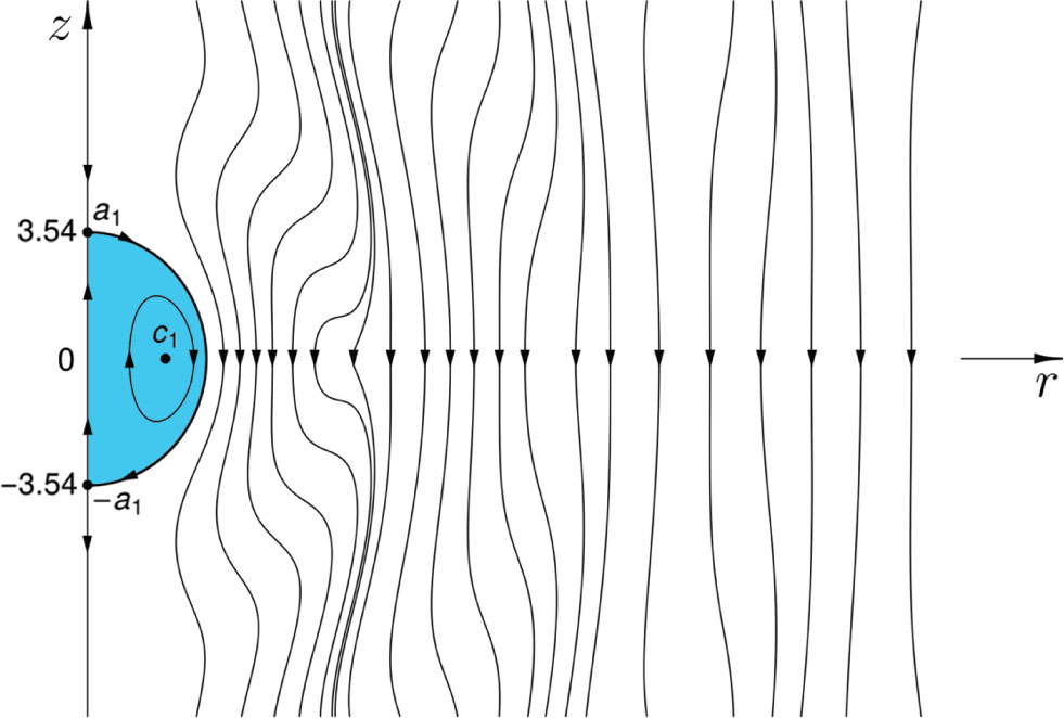
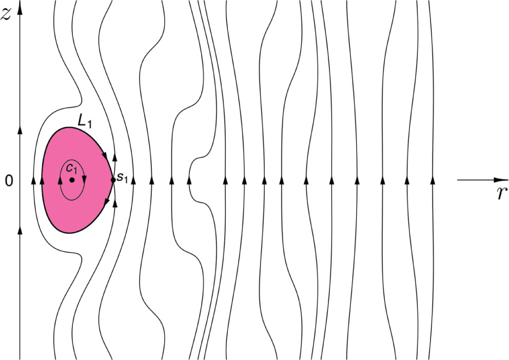
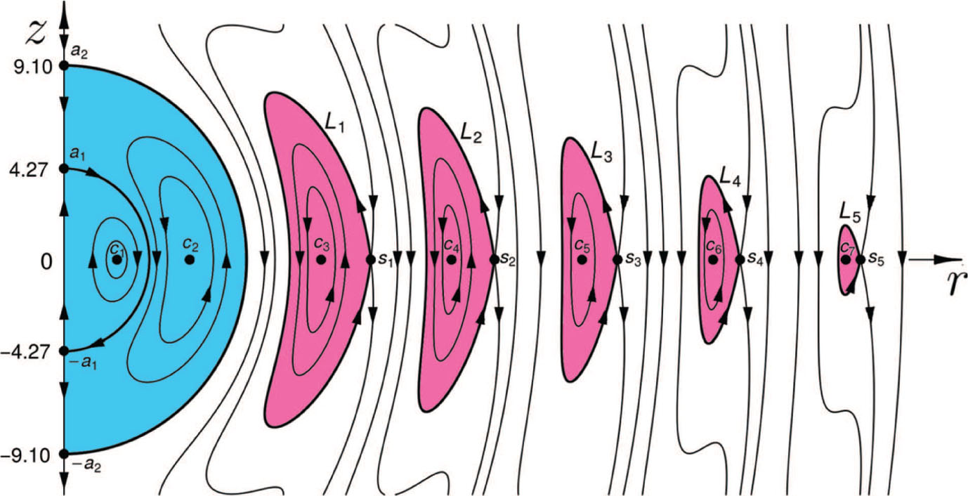
Figure 1 shows poloidal sections of magnetic surfaces ψ(r,z)=const for plasma equilibrium (3), (16) with ξ=−0.0237 and α = 1. They are up-down symmetric because flux function (16) satisfies the identity ψ(r,z)=ψ(r,−z). This equilibrium has three B,J-invariant maximal magnetic rings and one B,J-invariant spheroid of radius a = 4.08. The rings are maximal in the sense that they are not contained in any bigger B,J-invariant rings.
We have shown in [21], that the range I* of function G2(u) is the segment [−1/3,ξ1≈0.02872]. For the special values of parameter ξ belonging to the range I* one can find such a number a that ξ=G2(αa). Then the flux function (16) takes the form
(18)ψH=r2[G2(αa)−G2(αR)].
The corresponding magnetic field B (3) has invariant spheroid 𝔹a of radius a with boundary sphere defined by the equation ψH(r,z)=0. In another form, the stream function (18) was first derived in 1899 in the pioneer paper by Hicks [22] that is the historical precursor of many works on fluid and plasma equilibria.
Remark 1Parameters α and ξ have the following physical meaning: parameter ξ defines the range of the safety factor q(ψ) for magnetic field B(α,ξ) in each of the B(α,ξ)-invariant spheroids 𝔹ak (for −1/3<ξ<ξ1≈0.02872,ξ=G2(αak)) and characterizes the deviation of magnetic field B(α,ξ) (3) from the spheromak magnetic field Bs [24], [25] that coincides with B(α,0). Parameter α specifies the scaling of the plasma equilibria B(α,ξ).
VII. Consider the special case of function ΦN(r,z) (13):
Φ1(r,z)=ξr2+1α2∂ψ(r,z)∂z=ξr2−1α2∂[r2G2(αR)]∂z.
Using formula (17) we find:
(19)Φ1(r,z)=r2[ξ−zG3(αR)],G3(u)=1u4[(3−u2)sinuu−3cosu].
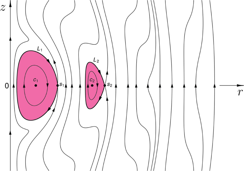
Figure 2 shows poloidal sections Φ1(r,z)=const of magnetic surfaces for magnetic field (3), (19) for ξ = 0.0075 and α = 1. Plasma equilibrium (3), (19) has three B,J-invariant maximal magnetic rings and three magnetic blobs. Flux function (19) and its magnetic surfaces Φ1(r,z)=const evidently are up-down asymmetric.
The general flux function Ψ2(r,z) (11) has the form
(20)Ψ2(r,z)=r2[ξ−G2(αR)+b1zG3(αR)+b2(G3(αR)+z2α2G4(αR))]
and is up-down asymmetric if b1≠0. Here function G4(u) has the form
G4(u)=1u6[(6u2−15)sinuu−(u2−15)cosu].
VIII. The electric current J for the magnetic field B (3) with w=𝒢(ψ) is
(21)μJ=curlB=−[𝒢(ψ)]zre^r+[𝒢(ψ)]rre^z−1r(ψrr−1rψr+ψzz)e^φ.
Remark 2Equations 3 and 21 yield that for the magnetic circulation w(r,z)=𝒢(ψ)=αψ and any flux functions ψ(r,z) satisfying (9) with ξ = 0 the magnetic field B (3) satisfies the Beltrami equation curlB=αB. Therefore, the flux functions ΨN(r,z) (11) and ΦN(r,z) (13) for ξ = 0 define an infinite-dimensional linear space of axisymmetric Beltrami fields (3). Lüst and Schlüter [26] were the first to study the axisymmetric Beltrami fields; exact formulas for them in terms of Bessel’s functions were derived by Chandrasekhar [25], see also [27]. The flux functions (11), (13), (16) and the corresponding to them Beltrami fields (3) have explicit form in terms of elementary functions, see formulas (19), (20), (40).
Remark 3In Section 5, we construct for infinitely many values ξk(k=1,2,3,⋯) of parameter ξ exact magnetic fields B(α,ξk) (3), (16) which are defined in a spheroid of certain radius ak and together with the pressure p vanish at the boundary sphere R=ak. The first eight values ξk are presented in (65) below. These solutions are continuously matched with empty space for R>ak and therefore have finite energy. For these solutions, the question of asymptotic behaviour at r → ∞ has no interest since they vanish for all R≥ak. For other values of parameter ξ≠ξk, k=1,2,3,⋯, magnetic field B(r,z) (3) and electric current J(r,z) (21) have the following asymptotics at r → ∞:
(22)B(r,z)≈2ξe^z+αξre^φ,J(r,z)≈2αξμ−1e^z.
Formulae (22) imply that electric current J(r,z) asymptotically is constant at r → ∞ and magnetic field lines asymptotically are helices lying on the vertical cylinders r = const. For ξ = 0 we get the spheromak magnetic field Bs(r,z) [25], [24] for which both Bs(r,z) and Js(r,z) tend to zero at r → ∞.
IX. We discuss simultaneously the plasma equilibria and fluid equilibria because they obey the equivalent equations [28]. The plasma equilibria corresponding to the Hicks hydrodynamic solutions (18) were presented in 1957 by Prendergast [29] in terms of Bessel’s functions. In this paper we use the definition of the pitch 𝒫 of helical curves (and the corresponding safety factor q=𝒫/(2π)) that is different from the Hicks’ [22] and Moffatt’s ones [30] and that is applicable to any axisymmetric fluid and plasma equilibria.
Hicks derived in [22] (4) for the steady axisymmetric stream functions ψ(r,z) that is widely known as the Grad–Shafranov equation [2], [3] because they independently rediscovered it 59 years later, in 1958. The same equation was rediscovered in 1950 by the aerospace engineers Bragg and Hawthorne [36] and in 1957 by Lüst and Schlüter [37]. Hicks presented in [22] the stream function that describes the spheromak Beltrami flow (with parameter λ = 0 (6)) that in 1958 was rediscovered in terms of Bessel’s functions by Woltjer [24] as a plasma equilibrium and by Chandrasekhar in [25] among many force-free axisymmetric plasma equilibria satisfying the linear Beltrami equation (2) with constant α. Hicks derived in [22] the conditions for vanishing of the corresponding to (18) flow on the boundary sphere 𝕊a2 rediscovered in 1957 by Prendergast [29]. Hicks’ fluid equilibria defined by the ψ functions (18) were rediscovered in 1969 by Moffatt [30] in terms of Bessel’s functions.
Remark 4As known, in the ideal hydrodynamics the vortex field curlV is frozen into the flow. We have shown in [21] that for the exact solutions (16), the properties of the hydrodynamic safety factor qh defined for the vortex field curlV are qualitatively different from the magnetohydrodynamic safety factor q investigated in the present paper. In [33], we studied vortex knots for the spheromak Beltrami fluid flow that has the stream function ψ=−r2G2(αR). We have derived exact formulas for the ranges of the rational numbers m/n that classify the vortex knots in all invariant spherical shells. In [34], the vortex knots are classified for another axisymmetric Beltrami flow that has stream function ψ=−zr2G3(αR) that is a special case for ξ = 0 of the flux function Φ1(r,z) (19). This flow has invariant plane z = 0 and invariant hemispheres 𝕊k+2, z ≥ 0, R=Rk and 𝕊k−2, z ≤ 0, R=Rk where Rk are roots of equation G3(αR)=0.
X. Plasma equilibria (3), (16) with parameter ξ outside the range I*, namely 0.02872<ξ<0.11182, possess several maximal B(α,ξ),J(α,ξ)-invariant magnetic rings ℛi3 that are bounded by toroidal magnetic surfaces and filled with nested magnetic surfaces isomorphic to tori 𝕋2 and having the innermost magnetic axes 𝕊i1. The rings are maximal in the sense that they are not contained in any bigger B,J-invariant rings. Equilibria (3), (16) with ξ∈[0.02872,0.11182] have no B,J-invariant spheroids, see Figure 3 for ξ = 0.0461.
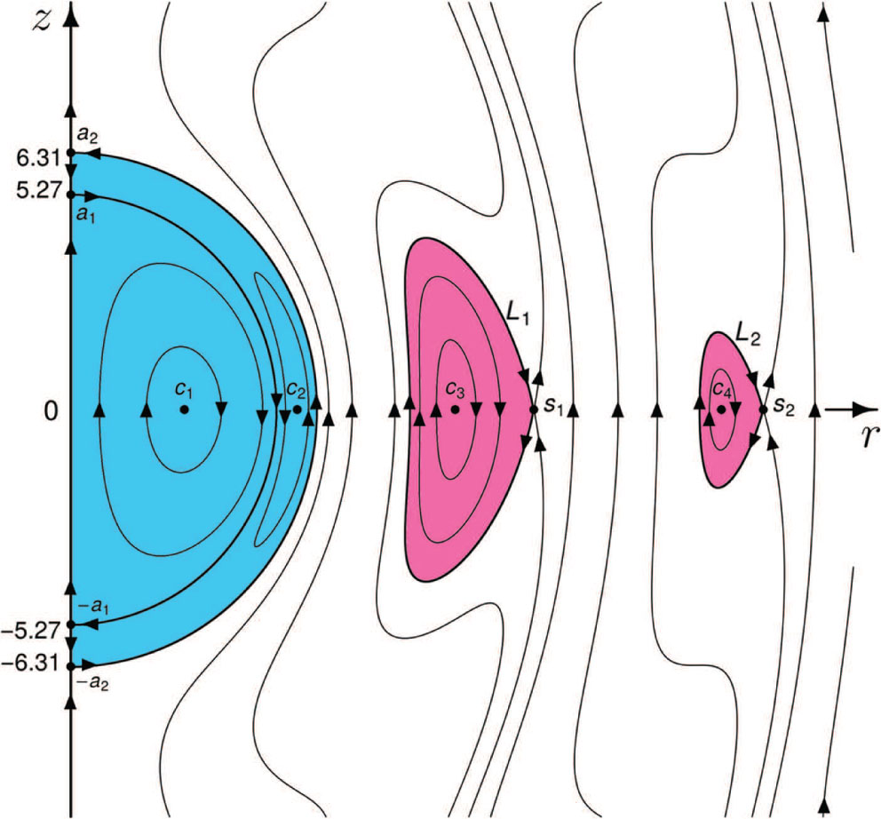
We show in Section 4 that all plasma equilibria (3), (16) with ξ belonging to the segment [−0.0648,0.02872], ξ ≠ 0, inside the range I* have several maximal B,J-invariant magnetic rings ℛi3 and several nested B,J-invariant spheroids 𝔹ak3, see Figures 1 and 4. We present in Section 5 equilibria (3), (16) with two and five maximal B(α,ξ),J(α,ξ)-invariant magnetic rings ℛi3, see Figures 5 and 6.
Remark 5Exact flux functions (11), (13), (15), (16) define plasma equilibria which for certain values of parameters ξ,bkn, zkn, k = 1, ⋯, M, n = 1, ⋯, N possess maximal magnetic rings, see Figures 1–7. These exact plasma equilibria can be used to study stability of controlled toroidal plasmas in cameras having shapes of the maximal magnetic rings. The pressure p has constant value (10) on the surface of a magnetic ring. The rings are invariant with respect to the magnetic field B (3) flux and the electric current J (21) flux.
Figure 8 demonstrates the poloidal contours for the force-free spheromak magnetic field (3) having the flux function (16) with ξ = 0 and collinear vector fields B and J satisfying Beltrami equation (2). The spheromak plasma equilibrium is qualitatively different from the non-force-free equilibria because for it the space ℝ3 is filled with infinitely many nested B(α,0)-invariant spheroids and there are no isolated maximal magnetic rings.
2 Exact Limit of the Safety Factor q(ψ) at a Magnetic Axis
I. Bellan derived in [13] the exact formula for the limit of the safety factor at a magnetix axis for the up-down symmetric plasma equilibria. In this section, we derive a generalization of Bellan’s formula [13] for the up-down asymmetric plasma equilibria.
Remark 6Plasma equilibria (3), (16) are up-down symmetric because flux function ψ(r,z) (16) satisfies identity ψ(r,z)=ψ(r,−z). The general equilibria (3), (11) and (3), (13) are up-down asymmetric if at least one coefficient b2k+1 is non-zero, see formulas (19), (20) and Figure 2. Plasma equilibria (3), (15) with generic constants zkn also are up-down asymmetric.
As known, integral curves x(t) of any vector field V(x) satisfy the equation dx(t)/dt=V(x(t)) [42]. Analogously the magnetic field B(x) lines (which by definition are integral curves of the vector field B(x)) in the cylindrical coordinates (r,z,φ) satisfy the equation
(23)dxdt=ddt(xe^x+ye^y+ze^z)=r˙e^r+rφ˙e^φ+z˙e^z=B(x).
Equation (23) by virtue of (3) and (5) takes the form of the system of three equations
(24)r˙=−1rψz,z˙=1rψr,
(25)φ˙=1r2𝒢(ψ).
Suppose that the flux function ψ(r,z) has a local non-degenerate maximum or minimum ψm=ψ(cm) at a point cm with coordinates (rm,zm):
(26)ψr(cm)=0,ψz(cm)=0,ℋm=ψrr(cm)ψzz(cm)−ψrz2(cm)>0.
Hence the system (24) has the center equilibrium point cm and system (24)–(25) has a closed trajectory – magnetic axis 𝕊m: r=rm, z=zm, 0≤φ<2π. All trajectories of system (24) near the center are closed curves Cψ: ψ(r,z)=const encircling the point cm. The corresponding trajectories of system (24)–(25) move on the invariant axisymmetric tori 𝕋ψ2=Cψ×𝕊1 (where circle 𝕊1 corresponds to the angle φ) and are either closed curves or everywhere dense on 𝕋ψ2 infinite helices.
Assume that a closed magnetic field line on a torus 𝕋ψ2 goes m times a long way (around the circle 𝕊1) and n times a short way (around the closed curve Cψ). A safety factor q for such a curve is defined [10], [11] by the formula q(ψ)=m/n and is the same for all magnetic lines on 𝕋ψ2 due to the axial symmetry. For the non-closed helical magnetic lines on 𝕋ψ2 a safety factor is q(ψ(t1))=limm/n when m,n→∞ along a given infinite curve.
We will use another definition of the safety factor that is equivalent to the above. Let t(ψ) be the period of the closed trajectory Cψ. A safety factor q(ψ) of the helices on the torus 𝕋ψ2 is equal to the increment of the angle φ during one period t(ψ), divided by 2π:
(27)q(ψ)=12π∫0t(ψ)dφdtdt.
Substituting (25) we get
(28)q(ψ)=𝒢(ψ)2π∫0t(ψ)dtr2(t).
Remark 7The safety factor q(ψ) is connected with the pitch 𝒫(ψ) of the helical magnetic field lines by the relation q(ψ)=𝒫(ψ)/2π. The term “pitch” was used in [22], [30], [31], [32].
In the limit ψ→ψm we have r(t)→rm for all t, hence (28) yields
(29)q(ψm)=limψ→ψmq(ψ)=t(ψm)𝒢(ψm)/(2πrm2),
where t(ψm)=limψ→ψmt(ψ).
II. The system of two (24) near the equilibrium point (rm,zm) is approximated by the system in variations [42]
(30)dδrdt=−a11δz−a12δr,dδzdt=a12δz+a22δr,
(31)a11=1rmψzz(cm),a12=1rmψrz(cm),a22=1rmψrr(cm),
where δr(t)=r(t)−rm, δz(t)=z(t)−zm. From (26), (31) we get
(32)Dm=a11a22−a122=1rm2ℋm>0.
Linear system (30) has quadratic first integral
Q(δr,δz)=a22(δr)2+2a12(δr)(δz)+a11(δz)2
that in view of (32) is either positive or negative definite. Hence its level curves Q(δr,δz)=const are nested ellipses and therefore all solutions to (30) are periodic. Due to the scaling invariance of system (30) all its solutions have the same period tm=2π/Dm.
From the general theory of differential equations [42] it follows that the limit at ψ→ψm of the function of periods t(ψ) is the period tm=2π/Dm of the system in variations (30). Using formula (32) we find:
(33)t(ψm)=limψ→ψmt(ψ)=2πDm=2πrmℋm.
Substituting (33) into (29) we get
(34)q(ψm)=limψ→ψmq(ψ)=𝒢(ψm)rmℋm.
Thus we have proved that for the case of arbitrary functions F(ψ), 𝒢(ψ) in the Grad–Shafranov equation (4) the safety factor q(ψ) has a finite and non-zero limit at ψ→ψm defined by formula (34) where ℋm=ψrr(cm)ψzz(cm)−ψrz2(cm)>0 (26).
The limit (34) is one of the two exact bounds for the range of the safety factor q(ψ).
Remark 8Bellan’s formula [13] for the safety factor at the magnetic axis is based on the assumption ∂2ψ/∂r∂z(cm)=0 that holds for the up-down symmetric plasma equilibria. Our formula (34) is valid for the general equilibria with ∂2ψ/∂r∂z(cm)≠0. For example, it is valid for the new exact up-down asymmetric plasma equilibria with the flux functions ΨN(r,z) (11) and ΦN(r,z) (13) where at least one coefficient b2k+1≠0 (see formulas (19), (20)) and for the equilibria with flux functions ΨN.M(r,z) (15) with generic constants zkn.
3 Magnetic Field B(α,ξ) in the First Invariant Spheroid
I. We will use the following elementary functions
(35)G0(u)=−cosu,G1(u)=duduG0(u)=sinuu,G2(u)=duduG1(u)=1u2(cosu−sinuu),G3(u)=duduG2(u)=1u4[(3−u2)sinuu−3cosu],
that are analytic everywhere and have the following limits at u → 0:
(36)G1(0)=1,G2(0)=−1/3,G3(0)=1/15.
Functions Gn(u) (35) are even and satisfy the identities
(37)G0(u)+G1(u)+u2G2(u)=0,G1(u)+3G2(u)+u2G3(u)=0.
The general identity
(38)Gn(u)+(2n+1)Gn+1(u)+u2Gn+2(u)=0,Gn+1(u)=u−1dGn(u)/du
follows from identities (37) by induction. Functions Gn(u) (35), (38) are connected with Bessel’s functions Jν(u) [43] of order ν=n−1/2 by the relations Gn(u)=π/2(−1)n−1Jn−1/2(u)/un−1/2.
II. Let us show that flux function ψ(r,z)=[ξ−G2(αR)]r2 satisfies (9). Indeed, using formulas (38) we find
ψr=2r[ξ−G2(αR)]−α2r3G3(αR),ψz=−α2r2zG3(αR),ψrr=2[ξ−G2(αR)]−5α2r2G3(αR)−α4r4G4(αR),ψzz=−α2r2G3(αR)−α4r2z2G4(αR).
Hence we get
(39)ψrr−1rψr+ψzz=−α2r2[5G3(αR)+(αR)2G4(αR)].
Identity (38) for n = 2 and u=αR takes the form
G2(αR)+5G3(αR)+(αR)2G4(αR)=0.
Substituting this identity into (39) we get
ψrr−1rψr+ψzz=α2r2G2(αR)=α2(ξr2−ψ).
Therefore the flux function ψ(r,z) (16) is an exact solution to (9).
III. Magnetic field B(α,ξ) (3), (16) has the following explicit form
(40)B(α,ξ)=α2rzG3(αR)e^r+[2[ξ−G2(αR)]−α2r2G3(αR)]e^z+α[ξ−G2(αR)]re^φ.
Substituting 𝒢(ψ)=αψ and formula (16) into the system (24), (25), we get:
(41)r˙=α2rzG3(αR),z˙=2[ξ−G2(αR)]−α2r2G3(αR),
(42)φ˙=α[ξ−G2(αR)].
Formula (40) for ξ = 0 describes the spheromak fluid flow Bs (satisfying Beltrami equation curlB=αB) that was discovered first by Hicks [22] in terms of elementary functions and half a century later was rediscovered by Woltjer [24] and Chandrasekhar [25] in terms of Bessell functions J3/2(αR) and J5/2(αR) as a force-free plasma equilibrium. The corresponding flux function ψ(r,z) was derived in [25], [24] in the form
(43)ψ(r,z)=r2A(aR)3/2J3/2(αR).
Hicks formula (18) with G2(αa)=0 coincides with the Chandrasekhar – Woltjer one (43) for A=π/2(αa)−3/2 in view of the formula for the Bessell function
J3/2(u)=−1π/2u(cosu−sinuu)=−1π/2u3/2G2(u)
that follows from [43], p. 56. The spheromak plasma equilibrium solution was studied (in terms of the Bessell functions) in [32], [44], [45], [46], [47], [27], [13], [48], see review [49]. The term “spheromak” was first introduced in [44].
IV. Suppose that parameter ξ belongs to the range of function G2(u). Then there exists such a minimal number a > 0 that ξ=G2(αa). Formula (18) yields that magnetic surface ψH(r,z)=0 contains the sphere 𝕊a2. Hence the whole spheroid 𝔹a3 where R ≤ a is invariant under the magnetic flux defined by the field B(α,ξ) (40).
The first root of equation G2(u)=0 is
(44)u=u¯1≈4.4931.
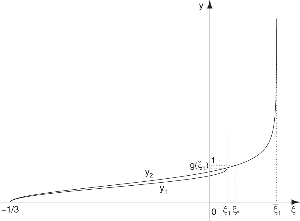
Figure 9 shows that the range of function y1(u)=G2(u) for all positive u is the segment I*: [−1/3,ξ1] where ξ1 is the maximal value of function G2(u). The maximum is attained at a point u1 where derivative G′2(u1) vanishes, ξ1=G2(u1). From (35) we get G3(u1)=u1−1G′2(u1)=0. The first root of equation G3(u)=0 is u1≈5.7635. Hence we find the value of ξ1=G2(u1)≈0.02872. Only for ξ∈I* equation
(45)G2(u)=ξ
has some solutions. Let g1(ξ) be the smallest solution to (45):
(46)G2(g1(ξ))=ξ.
We will use also function
(47)g(ξ)=g1(ξ)/(2π).
Both functions g1(ξ) and g(ξ) are defined on the segment I*: [−1/3,ξ1≈0.02872] and monotonously increase from g1(−1/3)=0 to g1(ξ1)=u1≈5.7635 and from g(−1/3)=0 to g(ξ1)=u1/(2π)≈0.9173.
Function y1(u)=G2(u) (35) near u = 0 has the form G2(u)≈−1/3+u2/30, see Figure 9. Therefore from (45) we find the asymptotics of function g1(ξ) at ξ→−1/3:
(48)g1(ξ)≈30ξ+1/3,g1(−1/3)=0.
The following values of function g1(ξ) will be used later:
(49)g1(0)=u¯1≈4.4931,g1(ξ1)=u1≈5.7635.
V. Magnetic field B(α,ξ) (40) for ξ∈I* has an invariant sphere 𝕊a2 of radius a=g1(ξ)/α on which it takes the form
(50)B~(α,ξ)=α2rG3(g1(ξ))[ze^r−re^z].
Hence the spheroid 𝔹a3 defined by the inequality R≤a=g1(ξ)/α is invariant under the magnetic flux (40).
Let us consider the Hill’s flux function [50]
ψa(r,z)=Cr2(1−a3R3),C=const,
that satisfies equation
(51)ψa,rr−1rψa,r+ψa,zz=0.
Hence function ψa(r,z) satisfies the Grad–Shafranov equation (4) with F(ψ)=0, 𝒢(ψ)=0. Therefore, the corresponding magnetic field (3) has w(r,z)=𝒢(ψ)=0 and takes the form
(52)Ba(r,z)=−3Crza3R5e^r+C[2(1−a3R3)+3r2a3R5]e^z.
Using (21), (51) and 𝒢(ψ)=0 we find Ja=curlBa=0. Hence magnetic field Ba (52) is current free.
On the sphere 𝕊a2(R=a) vector field (52) becomes
(53)B~a=−3Ca2r[ze^r−re^z].
Vector field (53) coincides with (50) when C=−13α2a2G3(αa). Therefore we assume that magnetic field B(α,ξ) (40) inside the invariant spheroid 𝔹a3 with a=g1(ξ)/α is continuously matched with the magnetic field Ba(r,z) (52) for C=−13α2a2G3(αa) outside the spheroid 𝔹a3. The magnetic field Ba(r,z) tends to a constant field 2Ce^z when R → ∞ and is current-free.
4 B(α,ξ)-invariant Rings and Spheroids
I. From Figure 9 it is evident that equation G2(u)=ξ (45) for ξ ≠ 0, ξ∈I*=(−1/3,ξ1≈0.02872) has a finite number N(ξ) of roots and N(ξ)→∞ when ξ → 0. That means the system (41)–(42) in the whole space ℝ3 can have for ξ ≠ 0 a finite number N(ξ) of invariant spheroids 𝔹ai3 and it has infinitely many invariant spheroids when ξ = 0. We consider system (41)–(42) in the first invariant spheroid 𝔹a13, a1=α−1g1(ξ), corresponding to the smallest root g1(ξ) of (45).
Figure 9 shows that (45) has no solutions if ξ<−1/3 or ξ>ξ1. Hence the magnetic field (40) does not have any invariant spheroids 𝔹c3(R≤c) if ξ<−1/3 or ξ>ξ1≈0.02872.
II. For ξ∈I* the system (41), (42) has at least one invariant spheroid 𝔹a13, a1=α−1g1(ξ). System (41) in the invariant semi-disk D1(ψ(r,z)≥0, r ≥ 0, R≤a1) has three equilibrium points: s1(r=0,z=a1), s2(r=0,z=−a1), c1(r=um/|α|, z = 0). The equilibria s1 and s2 are non-degenerate saddles if G3(g1(ξ))≠0. Their separatrices are: the interval I1:(r=0,−a1<z<a1) and the arc S1:(r2+z2=a12,r>0), see Figure 10. The equilibrium c1 is a center, its coordinate r=Rm=um(ξ)/α, where um(ξ) is the first positive root of equation 2G2(u)+u2G3(u)=2ξ (i.e. condition that z˙=0 in (41) at the point (r=α−1u,z=0)). The latter in view of the second identity (37) takes the form
(54)y2(u)=−[G1(u)+G2(u)]/2=ξ.
All equilibrium points of system (41) with r ≠ 0 are (rk(ξ)=α−1uk(ξ),z=0) where uk(ξ) is a root of (54). The first root of equation G1(u)+G2(u)=0 is
(55)um(0)=v¯1≈2.7437,
see Figure 9 for the plot of function y2(u)=−[G1(u)+G2(u)]/2.
III. It is evident from Figure 9 that for 0<ξ<ξ¯1 solutions to (54) appear in pairs u2k−1(ξ)<u2k(ξ), k = 1, 2, ⋯ , N. From the plots of functions y1(u)=G2(u) and y2(u)=−[G1(u)+G2(u)]/2 in Figure 9 it follows that the amplitudes of the subsequent oscillations of function −[G1(u)+G2(u)]/2 are greater than those of G2(u). Therefore if uℓ(ξ) is the maximal solution to (45), then (54) has several pairs of solutions u2k−1(ξ)<u2k(ξ) that are greater than uℓ(ξ). The u2k−1(ξ) defines a magnetic axis with coordinates r=α−1u2k−1(ξ),z=0,0≤φ≤2π that is a stable closed trajectory of system (41), (42). The points u2k(ξ) define the unstable closed trajectory r=α−1u2k(ξ),z=0,0≤φ≤2π of system (41), (42). The stable (with respect to the system (41), (42)) magnetic axis lies inside the B(α,ξ)-invariant isolated magnetic ring ℛi3 and the unstable one lies on its toric boundary. For all roots uj(ξ) of (54) satisfying uj(ξ)<uℓ(ξ), equations r=α−1uj(ξ),z=0,0≤φ≤2π define stable magnetic axes 𝕊j1 inside the largest B(α,ξ)-invariant spheroid 𝔹aℓ3 where aℓ=α−1uℓ(ξ).
For −1/3<ξ<0 the plot of function y2(u)=−[G2(u)+G3(u)]/2 in Figure 9 shows that the smallest solution u=umin(ξ) to (54) satisfies
umin(ξ)<v¯1≈2.7437<u¯1≈4.4931,
where (44) and (55) are used and u¯1 is the first root (44) of equation G2(u)=0. Therefore the corresponding magnetic axis r=α−1umin(ξ),z=0,0≤φ≤2π lies inside the first B(α,ξ)-invariant spheroid 𝔹a13 and is Tables. The other solutions to (54) appear in pairs u2m(ξ)<u2m+1(ξ), m=1,2,⋯ and the above description is applicable. If uℓ(ξ) is the maximal solution to (45), then each pair u2m(ξ)<u2m+1(ξ) with u2m(ξ)>uℓ(ξ) defines a B(α,ξ)-invariant isolated magnetic ring ℛi3 where the u2m(ξ) defines a stable (with respect to the system (41), (42)) magnetic axis and the u2m+1(ξ) defines the unstable one.
The presented arguments and the plots in Figure 9 prove that all magnetic fields B(α,ξ) (40) with ξ¯2<ξ<ξ¯1 possess several isolated magnetic rings. Here ξ¯2≈−0.0648 and ξ¯1≈0.11182, see formulas (57) below and Figure 9.
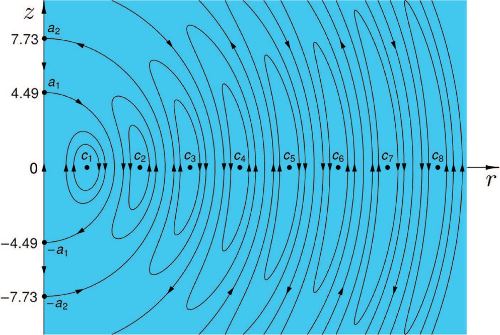
IV. From Figure 9 it follows that the range of function y2(u)=−[G1(u)+G2(u)]/2 for all positive u is the segment [−1/3,ξ¯1] where ξ¯1 is its maximum that is attained at a point v1; hence we have G′1(v1)+G′2(v1)=0. Equations (35) yield G′1(u)+G′2(u)=u[G2(u)+G3(u)]; therefore G2(v1)+G3(v1)=0. The first root of this equation is v1≈4.2329. Hence, we get ξ¯1=−2−1[G1(v1)+G2(v1)]≈0.11182.
The first seven zeros of function G2(u)+G3(u) are
(56)v1=4.2329,v2=7.5896,v3=10.8103,v4=13.9941,v5=17.1622,v6=20.3219,v7=23.4767.
These points are local maxima and minima of the function y2(u)=−[G1(u)+G2(u)]/2, see Figure 9. The corresponding values of function y2(u) are
(57)y2(v1)=ξ¯1=0.11182,y2(v2)=ξ¯2=−0.0648,y2(v3)=ξ¯3=0.0459,y2(v4)=ξ¯4=−0.0355,y2(v5)=ξ¯5=0.0290,y2(v6)=ξ¯6=−0.0245,y2(v7)=ξ¯7=0.0213.
Values (57) give for the local maxima of function y2(u)=−(G1(u)+G2(u))/2:
ξ¯1>ξ¯3>ξ¯5>ξ1≈0.02872;ξ1>ξ¯7.
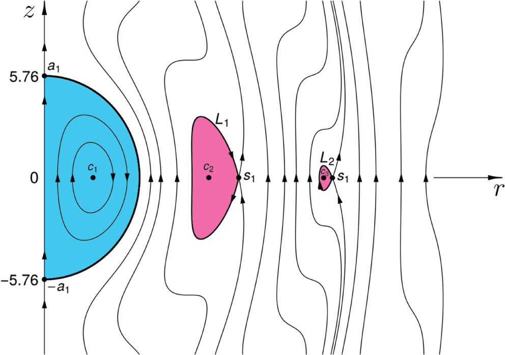
These inequalities imply that for ξ1<ξ<ξ¯5 there are three B(α,ξ)-invariant isolated magnetic rings ℛi3⊂ℝ3. For ξ¯5<ξ<ξ¯3 there are two B(α,ξ)-invariant rings ℛ13, ℛ23, see Figure 7 in Section 1, where ξ = 0.0326. For ξ¯3<ξ<ξ¯1 there is one B(α,ξ)-invariant isolated magnetic ring ℛ13⊂ℝ3.
V. The extremal values of function y1(u)=G2(u) are attained at zeros of function G3(u)=u−1G′2(u). The first eight of them are
(58)u1=5.7635,u2=9.0950,u3=12.3229,u4=15.5146,u5=18.6890,u6=21.8539,u7=25.0128,u8=28.1678.
The corresponding local maxima and minima of function y1(u)=G2(u) are (Fig. 9)
(59)G2(u1)=ξ1=0.02872,G2(u2)=ξ2=−0.0119,G2(u3)=ξ3=0.0065,G2(u4)=ξ4=−0.0041,G2(u5)=ξ5=0.0029,G2(u6)=ξ6=−0.0021,G2(u7)=ξ7=0.0016,G2(u8)=ξ8=−0.0013.
Values (57) and (59) imply for the local minima of function y2(u)=−(G1(u)+G2(u))/2:
ξ¯2<ξ¯4<ξ¯6<ξ2≈−0.0119.
From Figure 9 we see that for −1/3<ξ<ξ2 magnetic field B(α,ξ) has only one invariant spheroid 𝔹a13 and a number of isolated magnetic rings ℛi3⊂ℝ3 depending on ξ. For ξ=ξ2≈−0.0119 there are five invariant magnetic rings ℛi, see Figure 6 in Section 1.
Equation (54) for ξ>ξ¯1 or ξ<−1/3 does not have any roots. Hence system (41) has no equilibrium points with r > 0 and no closed trajectories. Therefore magnetic field B(α,ξ) (40) has no invariant tori 𝕋2 and no closed magnetic field lines for ξ>ξ¯1 or ξ<−1/3.
5 Applications to the Magnetic Star Model
I. Chandrasekhar and Fermi [51] and Prendergast [29] have proposed a model of magnetic star where it was supposed that plasma velocity vanishes: V(x)≡0. In this section we present a generalization of the Chandrasekhar, Fermi and Prendergast model where dynamics of plasma is included. As in [51], [29], we suppose that the star has form of a spheroid 𝔹a3 of radius a with constant mass density ρ. Additionally we assume that the plasma velocity V(x) and magnetic field B(x) are collinear: V(x)=γB(x) where γ = const and that the boundary conditions
(60)V(x)=0,B(x)=0,p(x)=0,gradp(x)=0
hold on the sphere 𝕊a2, |x|=a. In this case, the plasma equilibrium inside the spheroid 𝔹a3 is continuously matched with the empty space for |x|>a, thus providing a model of magnetic star with dynamics of plasma inside it.
As known, for V(x)=γB(x) the steady equations of ideal magnetohydrodynamics (viscosity ν = 0 and plasma diffusivity η = 0) are reduced to
(61)(γ2ρμ−1)curlB×B=−grad(μp+γ2ρμ2|B|2+ρμΦ),divB=0,
where Φ(x) is the Newtonian gravitational potential. It is evident that (61) with pressure
(62)p=(1−γ2ρμ)p~−γ2ρ2|B|2−ρΦ+C1
take the form of (1): J×B=gradp~. Therefore, all previous results concerning the plasma equilibrium (1) are applicable to the more general magnetohydrodynamic equilibria (61) with γ≠±1/ρμ.
II. Consider magnetic field B(α,ξ) (40) defined by the flux function (16) where constant ξ∈I*=[−1/3,0.02872]. Here I* is the range of function G2(u) [21]. Then there exists such parameter αa that ξ=G2(αa). The magnetic surface ψ(r,z)=[G2(αa)−G2(αR)]r2=0 (18) evidently contains the sphere 𝕊a2: R = a and plasma pressure p~(r,z)=−ρα2ξμ−1ψ(r,z) (10) vanishes on 𝕊a2.
For ξ=G2(αa), magnetic field B(α,ξ) (40) on the sphere R = a takes the form
(63)B(α,ξ)=α2rG3(αa)[ze^r−re^z]
((63) coincides with (50) because G2(g1(ξ))=ξ). Therefore, the boundary conditions (60) are satisfied if
(64)ξ=G2(αa),G3(αa)=0.
Since G3(u)=u−1dG2(u)/du we get from (64) that the points αa are the points of extrema of function G2(u). From Figure 9 we see that the point αa is a local maximum of function y1(u)=G2(u) if G2(αa)>0 and it is a local minimum if G2(αa)<0.
III. To find solutions to (64) we use calculation (58) of the first eight roots of equation G3(u)=0. The corresponding radii of invariant spheroids 𝔹ak3 are ak=α−1uk. Calculating the values of function G2(u) at the points uk (58) we find the first eight values ξk=G2(uk)=G2(αak):
(65)ξ1≈0.02872,ξ2≈−0.0119,ξ3≈0.0065,ξ4≈−0.0041,ξ5≈0.0029,ξ6≈−0.0021,ξ7≈0.0016,ξ8≈−0.0013.
For ξ=ξk (65) and the corresponding values αak=uk (58) both (64) are satisfied. Hence we get that on the boundary sphere 𝕊ak2 magnetic field B(α,ξk)(r,z) (63) and plasma velocity V(r,z)=γB(α,ξk)(r,z) are identically zero.
Therefore, the magnetic field (40) and the plasma velocity can be continuously matched with the zero fields in the outer space R≥ak.
The plasma pressure p(x) is defined by formula (62) where p~(r,z)=−ρα2ξμ−1ψ(r,z) vanishes on the sphere 𝕊a2. Both plasma velocity V(x) and magnetic field B(α,ξk)(r,z) vanish on 𝕊a2. The gravitational potential Φ(x)=4π|x| is contant on the sphere 𝕊a2: Φ(x)=Φ(ak)=4πak since the density ρ is constant inside the spheroid 𝔹ak3. Therefore, the choice of constant C1=ρΦ(ak) in (62) yields p(x)=0 on the sphere 𝕊ak2. Hence the boundary conditions (60) are satisfied and the magnetic field B(α,ξk)(r,z) (40), plasma velocity V(α,ξk)(r,z)=γB(α,ξk)(r,z) and the pressure
(66)p=(γ2ρμ−1)ρα2ξμ[G2(αak)−G2(αR)]r2−γ2ρ2|B|2−ρΦ(R)+ρΦ(ak)
inside the spheroid 𝔹ak3 are continuously matched with the empty space outside of it, thus giving a model of a magnetic star with dynamics of plasma inside it.
6 The Limit of the Safety Factor at a Magnetic Axis and Function h(ξ)
I. Let us derive the exact formula for the limit of the safety factor q(ψm(ξ)) (34) for solutions (16) with ξ belonging to the range J* of function −[G1(u)+G2(u)]/2, that means ξ∈J*=[−1/3,ξ¯1≈0.11182]. Substituting r2=R2−z2 into formula (16) and using the first identity (37) for u=αR we find
(67)ψ(r,z)=ξr2+1α2[G0(αR)+G1(αR)]+z2G2(αR).
Differentiating function ψ(r,z) (67) and using formulas (35) we get
(68)∂ψ∂r=r[2ξ+G1(αR)+G2(αR)+α2z2G3(αR)],
∂ψ∂z=z[G1(αR)+3G2(αR)+α2z2G3(αR)].
Function ψ(r,z) (16) achieves its local maximal value ψm(ξ) at the point c1(ξ)=(rm(ξ),zm(ξ)). Since ψr(c1(ξ))=0, ψz(c1(ξ))=0, we get from (68): zm(ξ)=0 and um(ξ)=αrm(ξ) satisfies (54) and is its smallest root. Hence rm(ξ) is the smallest radius of all existing magnetic axes. For the second derivatives of function ψ(r,z) at the point c1(ξ) we find from (68)
ψrr(c1(ξ))=um2(ξ)[G2(um(ξ))+G3(um(ξ))],ψzz(c1(ξ))=G1(um(ξ))+3G2(um(ξ)),
and ψrz(c1(ξ))=0. Applying the second identity (37) we get ψzz(c1)=−um2G3(um). Hence we get for the Hessian (26)
(69)ℋm=−um4(ξ)G3(um(ξ))[G2(um(ξ))+G3(um(ξ))].
Let us show that ℋm>0. Equation (54) for ξ=ξ¯1≈0.11182 has the root um(ξ¯1)=v1≈4.2329<g1(0)=u¯1≈4.4931, where G2(u¯1)=0. Hence we get G2(um(ξ¯1))=G2(v1)<0. Numerical calculation gives G2(v1)≈−0.0140. Since G2(u) is monotonously increasing function of u∈[−1/3,u1≈5.7635] we find G3(um(ξ))=um−1(ξ)G′2(um(ξ))>0. Since −[G2(u)+G3(u)]=−u−1[G′1(u)+G′2(u)] and function y2(u)=−12[G1(u)+G2(u)] is monotonously increasing for u∈[0,v1≈4.2329] (see Figure 9), we find that −[G2(um(ξ))+G3(um(ξ))]>0. Hence we get from (69) ℋm>0.
Substituting into (34) formulas (69), αrm(ξ)=um(ξ) and 𝒢(ψm(ξ))=αψm(ξ)=αrm2(ξ)[ξ−G2(um(ξ))], we find for the exact solutions (16)
(70)h(ξ)=limψ→ψm(ξ)q(ψ)=ξ−G2(um(ξ))um(ξ)−G3(um(ξ))[G2(um(ξ))+G3(um(ξ))].
II. It is evident that expression (70) is a function of parameter ξ only, since um(ξ) is function of ξ defined as the smallest root of (54). Function h(ξ)=𝒢(ψm(ξ)) (70) describes one of the two boundaries of the range of the fractions m/n that correspond to the torus knots Km,n realised by the magnetic field lines for the magnetic field (40) defined by the flux function ψ(r,z) (16) for a given ξ∈J*=[−1/3,ξ¯1≈0.11182].
From Figure 9 it follows that ξ−G2(um(ξ))≥0 for ξ∈[−1/3,ξ¯1]. Hence we get that h(ξ)≥0 for ξ∈[−1/3,ξ¯1].
III. The limits (36) give −12[G1(0)+G2(0)]=−1/3. Hence we get from (54) um(−1/3)=0, that is evident also from Figure 9. Near u = 0 we have from (35) G1(u)≈1−u2/6 and G2(u)≈−1/3+u2/30. Hence (54) becomes um2(ξ)≈15(ξ+1/3). Therefore
(71)ξ−G2(um(ξ))≈ξ+1/3−um2(ξ)/30≈12(ξ+1/3).
Since G3(0)=1/15 and G2(0)+G3(0)=−4/15 we find from (70), (71) h(−1/3)=0 and get the asymptotics
(72)h(ξ)≈(15/4)ξ+1/3,ξ→−1/3.
IV. The point um(ξ¯1)=v1 is the point of maximum of function y2(u)=−[G1(u)+G2(u)]/2, see Figure 9. Hence we get from (35) G2(v1)+G3(v1)=v1−1[G′1(v1)+G′2(v1)]=0 and for um(ξ)≈v1 we have G2(um(ξ))+G3(um(ξ))≈v1[G3(v1)+G4(v1)](um(ξ)−v1). Therefore, using Taylor expantion we get that (54) near ξ¯1 takes the form ξ¯1−ξ≈14v12[G3(v1)+G4(v1)](um(ξ)−v1)2. Substituting this into (70) we find the asymptotics
(73)h(ξ)≈ξ¯1−G2(v1)v12G3(v1)[G3(v1)+G4(v1)]1/4(ξ¯1−ξ)1/4,ξ→ξ¯1.
Substituting ξ¯1≈0.11182, v1≈4.2329, G2(v1)=−G3(v1)≈−0.0140 and G4(v1)≈−0.0031 into (73) we get the formula
(74)h(ξ)≈0.5498(ξ¯1−ξ)−1/4→∞,ξ→ξ¯1.
Using (49) and substituting the values um(0)=v¯1≈2.7437 and um(ξ1)=u*≈2.9570 into formula (70) we get for ξ = 0 and ξ=ξ1≈0.02872:
(75)g(0)≈0.7152,q(ψm(0))=h(0)≈0.82524,
(76)g(ξ1)≈0.9173,q(ψm(ξ1))=h(ξ1)≈0.9305.
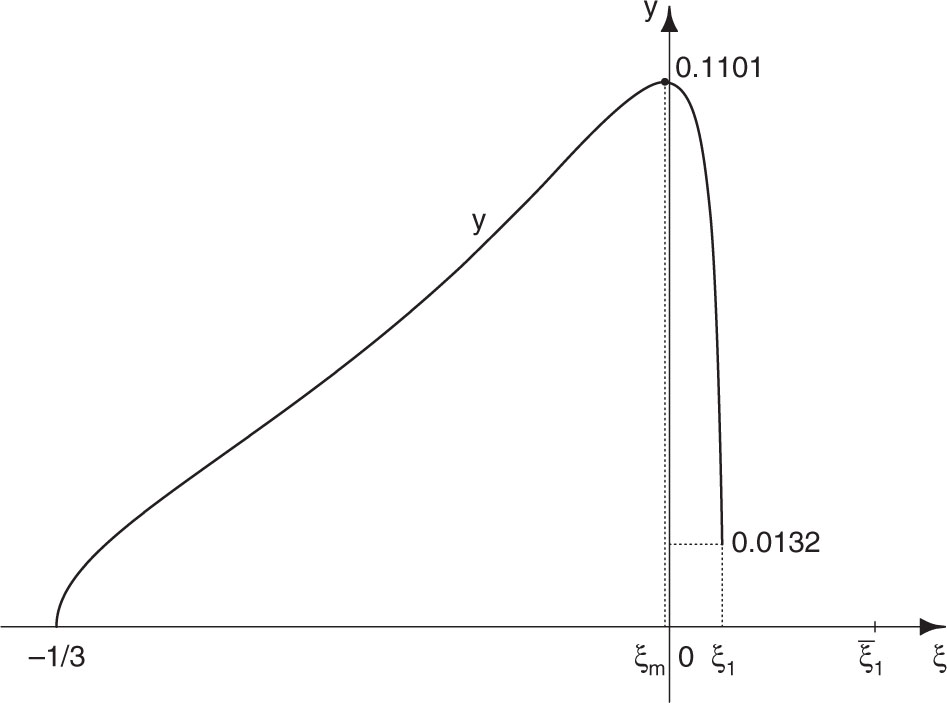
The plots of functions h(ξ) and g(ξ)=g1(ξ)/(2π) (47) are shown in Figure 11. All values of the safety factor q(ψ) inside the first invariant spheroid Ba13 belong to the interval (g(ξ),h(ξ)) that has the length ℓ(ξ)=h(ξ)−g(ξ). The maximal length ℓmax=ℓ(ξm)≈0.1101104 is achieved at ξm≈−0.0024483 and the zero length is the limit of ℓ(ξ) at ξ→−1/3. For the spheromak magnetic field B(α,0) we find from (75) ℓ(0)≈0.11002. For ξ=ξ1 we get from (76) ℓ(ξ1)≈0.0132. At the point ξ* we have h(ξ*)=1.
The plot of function ℓ(ξ) is presented in Figure 12. In Figures 11 and 12 two different scales of variable y are used that have the ratio 1:35.
7 The Limit of the Safety Factor q(ψ) at ψ → 0
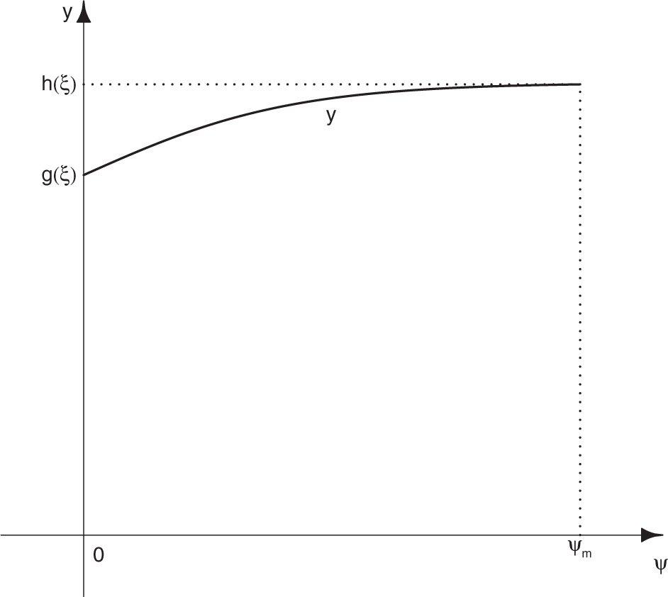
I. All trajectories of system (41) for −1/3<ξ≤ξ1 inside domain D1 are closed curves Cψ:ψ(r,z)=ψ=const, 0<ψ<ψm(ξ), encircling the center equilibrium point c1(ξ) and having periods t(ψ), see Figure 10. The corresponding trajectories of system (41)–(42) are helices moving on invariant tori 𝕋ψ2=Cψ×𝕊1⊂ℝ3 (circle 𝕊1 corresponds to the angle φ). In view of (42), the corresponding safety factor q(ψ) (27) is
(77)q(ψ)=12π∫0t(ψ)dφdtdt=α2π∫0t(ψ)[ξ−G2(αR(t))]dt.
For ξ∈I*, the closed trajectories Cψ at ψ → 0 approach the cycle of two separatrices I1 and S1 that satisfy equation ψ(r,z)=0, see Figure 10. Since dynamics along each separatrix takes an infinite time [42] we get limψ→0t(ψ)=∞. Therefore, the integral (77) contains an uncertainty because at the points s1(0,a1), s2(0,−a1) and on the semi-circle S1(r2+z2=a1) we have ξ−G2(αR(t))=0, where a1=g1(ξ)/α. To resolve this uncertainty we use the invariance of the safety factor q(ψ) (27) under the reparametrization of time t. After the change of time
dτdt=α[ξ−G2(αR)]
the system (41)–(42) turns into the system
(78)drdτ=αrzG3(αR)ξ−G2(αR),dzdτ=2α−1−αr2G3(αR)ξ−G2(αR),
(79)dφdτ=1.
On the invariant segment I1(r=0,−a1<z<a1), system (78) has the form dr/dτ=0, dz/dτ=2α−1. Dynamics of a trajectory along the segment I1 from point s2(0,−a1) to point s1(0,a1) takes time τ1≈2a1/(2α−1)=αa1=g1(ξ). Dynamics of a trajectory along the semicircle R=a1 from point s1(0,a1) to s2(0,−a1) takes infinitesimaly small time τ2≪1 because the speed of system (78) dynamics near the circle ξ−G2(αR)=0 tends to infinity.
Hence the total time τ0=τ1+τ2 of travel along the closed curve Cψ has the limit αa=g1(ξ) at ψ → 0. During this time the total change of the angle φ is g1(ξ) because dφ/dτ=1, see (79). Hence we get for the limit of the safety factor (77): limψ→0q(ψ)=g(ξ)=g1(ξ)/(2π). The continuity of the function q(ψ) implies that for ξ∈[−1/3,ξ1] the safety factor q(ψ) takes all values between the two limits q(0)=g(ξ) and q(ψm)=h(ξ). Numerical calculations performed in [33] demonstrate that the safety factor q(ψ) is a monotonous function of ψ, see Figure 5 of [33]. Such a monotonicity implies that the safety factor q(ψ) is changing strictly inside the limits
(80)g(ξ)<q(ψ)<h(ξ).
For example for ξ = 0 we get from (75):
(81)0.7152≈g(0)<q(ψ)<h(0)≈0.8252.
The numerical calculations of the functions h(ξ) and g(ξ)=g1(ξ)/(2π) are presented in their plots in Figure 11 that shows that g(ξ)≤h(ξ) for all ξ∈I*=[−1/3,ξ1≈0.02872]. Hence we get that for the magnetic field knots Km,n realized for ξ∈I* the following inequalities hold
(82)g(ξ)<mn<h(ξ).
Formulas (48) and (72) imply that the functions g(ξ) and h(ξ) have the following asymptotics at ξ→−1/3:
(83)g(ξ)≈302πξ+1/3,h(ξ)≈154ξ+1/3.
Here g(ξ)<h(ξ) because 30/(2π)≈0.8717<0.9682≈15/4.
The plot of the safety factor q(ψ) is shown in Figure 13. For example, for the spheromak magnetic field (ξ = 0) we find from (81) that only those magnetic field knots Km,n are realized for which the fractions m/n belong to the narrow gap of width ≈ 0.11002 defined by the inequalities 0.7152≈g(0)<m/n<h(0)≈0.8252.
8 Safety Factor q(ψ) for ξ1<ξ<ξ¯1
I. For ξ>ξ¯1 or ξ<−1/3 both (45) and (54) have no solutions, see Figure 9. Therefore, system of two (41) has no equilibrium points and no closed trajectories. For all its trajectories at t→±∞ we have z→±∞ and r→|ψ/ξ|. Hence magnetic fields (3), (16) for ξ>ξ¯1 or ξ<−1/3 have no invariant tori 𝕋2 and no closed magnetic lines.
II. For ξ1<ξ<ξ¯1, (45) does not have any roots. Hence function ψ(r,z)=r2[ξ−G2(αR)] is positive for r ≠ 0 and therefore the magnetic flux defined by formulas (3), (16) does not have any invariant spheroids 𝔹c3. Equation 54 for ξ1<ξ<ξ¯1 has (in general position) an even number of roots uci(ξ)=αrci(ξ) and usi(ξ)=αrsi(ξ), uci(ξ)<usi(ξ), see Figure 9. Therefore the corresponding system of two (41) has an even number of equilibrium points: the stable centers ci(r=rci(ξ),z=0) and the unstable saddles si(r=rsi(ξ),z=0). Each saddle equilibrium si has a loop separatrix Li which has its beginning and its end at the point si and satisfies equation
ψ(r,z)=r2[ξ−G2(αR)]=ψsi(ξ)=rsi2(ξ)[ξ−G2(usi(ξ))]=const>0.
The phase portrait of system (41) for ξ = 0.0326 is shown in Figure 7, where rc1=3.0263, rs1=5.6597 and rc2=10.1960, rs2=11.4485. The loop separatrices L1 and L2 bound invariant domains 𝒟1 and 𝒟2 that are filled with closed trajectories Cψ(ψ(r,z)=const) that define invariant tori of system of three (41), (42) 𝕋ψ2=Cψ×𝕊1⊂𝒟2×𝕊1. Here the circle 𝕊1 corresponds to the angle variable 0≤φ≤2π. The closure of the product 𝒟i×𝕊1 is the invariant ring ℛi3⊂ℝ3, i = 1,2.
All magnetic field knots for the system (41), (42) are contained in the rings ℛi3 because all trajectories of system (41) outside of the domains 𝒟i are infinite curves, see Figure 7.
The limit of the safety factor q(ψ) at ψ→ψmi(ξ)=ψ(ci(ξ)) has the form q(ψmi(ξ))=hi(ξ)>0 and is given by formula (70) where coordinate uci(ξ) is substituted instead of um(ξ). Closed trajectories Cψ⊂𝒟i have period t(ψ) and for ψ→ψsi(ξ) approach the loop separatrix Li. As known [42], dynamics along a loop separatrix takes an infinite time. Therefore, limψ→ψsi(ξ)t(ψ)=∞. Equation 28 with 𝒢(ψ)=αψ yields for any closed trajectory Cψ:
q(ψ)=αψ2π∫0t(ψ)dtr2(t).
Since 1/r2(t)>1/rsi2(ξ) for all t and limψ→ψsi(ξ)t(ψ)=∞ we get
q(ψsi(ξ))=limψ→ψsi(ξ)q(ψ)>α2πrsi2(ξ)limψ→ψsi(ξ)(ψt(ψ))=∞.
This result implies that the safety factor q(ψ) in the domain 𝒟i is continuously changing in the limits
hi(ξ)<q(ψ)<∞.
Therefore for the corresponding magnetic field knots Km,n we have
(84)hi(ξ)<mn<∞.
Formula (74) yields the asymptotics h1(ξ)≈0.5498 (ξ¯1−ξ)−1/4→∞ at ξ→ξ¯1.
The equilibria ci(ξ) and si(ξ) define respectively the stable (with respect to the system (41), (42)) and the unstable magnetic axes of the magnetic field (3), (16).
9 Comments on Hicks’ Papers
I. Hicks studied in [22], [23] fluid equilibria defined by the stream function
(85)ψH=A(J2(λra)−r2a2J2(λ))sin2θ,J2(u)=sinuu−cosu,
presented on pp. 34, 61. Here r=x2+y2+z2, θ is the polar angle, a the spherical aggregate’s radius. On p. 34 of [22] Hicks wrote:
“The most striking and remarkable fact brought out is that with increasing parameterλ, we get a periodic system of families of aggregates. ⋯ Of these families two are investigated more in detail than the others. In one family (theλ2family) all the members remain at rest in the surrounding fluid. In the other (theλ1family) the distinguishing feature common to all the members is that the stream lines and the vortex lines are coincident.”
On p. 69 Hicks continued:
“We shall call the values ofλcorresponding to the Q points theλ2values and denote them in order byλ2(1),λ2(2),⋯λ2(n). ⋯⋯Atλ=λ2(1)the aggregate is at rest, the velocity of the fluid on the boundary is zero.”
Therefore, the λ2 family is the countable set of solutions (85) for that the fluid velocity vanishes on the boundary sphere r = a. The corresponding values of λ=λ2(n) are roots of equation cotλ=λ−1−λ/3 [22], p. 74. These solutions were rediscovered in 1957 by Prendergast [29].
Also on p. 69 Hicks wrote:
“So we get another family formed by values ofλ, corresponding to points where the J-curve cuts the axis of x. We will call values ofλ, corresponding to these theλ1parameters, and denote the orders in the same way as for theλ2parameters. As we shall see shortly, the distinguishing property of this family is that in each of them the vortex lines and the stream lines coincide.”
Therefore, the λ1 family is the countable set of solutions (85) where λ=λ1(n) that are roots of equation J2(λ)=0 equivalent to tanλ=λ [22], p. 73. For these solutions the stream function (85) takes the form
(86)ψH=AJ2(λ1(n)r/a)sin2θ.
Solutions (86) were rediscovered by L. Woltjer in 1958 in terms of Bessel’s functions [24] and by S. Chandrasekhar [25] in 1956 among many other axisymmetric force-free plasma equilibria. The whole family λ1(n) actually describes the same spheromak Beltrami flow that is altered by the scaling parameter λ1(n). As the result of the scaling by λ1(n), solution (86) has n − 1 nested invariant subspheroids inside the invariant spheroid r = a.
The solutions (86) describe the spheromak Beltrami field that corresponds to solution (16) with ξ = 0.
Hence we see that Hicks had investigated not all solutions (85) but only the two subsets defined by the concrete values of λ2(n) and λ1(n) of which only 4 solutions defined by λ2(1),λ2(2),λ1(1),λ1(2) were analyzed, see pp. 93–94 of [22]. These solutions coincide with solutions (16) for three values of parameter ξ: ξ1≈0.02872, ξ2≈−0.0119 and ξ = 0.
II. On p. 72 Hicks presented his definition of the pitch:
“The total angular pitch of the spiral is
λ∫x1x2dxcosθ
where x1, x2are the two roots of
J(λx)−x2J(λ)=λψ(Siλ−sinλ)πμa=b,Siλ=∫0λsinyydy.”
The Hicks’ definition is applicable only to the considered solutions (85). Hicks did not present any definition of the pitch for a general axisymmetric fluid equilibria.
Using his definition of pitch, after long calculations on pp. 72–92 Hicks formulates on p. 93 his main results for solutions with parameter λ2(1)=5.7637 that corresponds to the value of our parameter ξ=ξ1≈0.02872:
“Angular pitch of stream lines at surface=330∘14′.
Angular pitch of stream lines at axis=334∘58′.
Angular pitch of vortex lines at axis=267∘.”
Dividing the Hicks’ values of pitch by 360∘ we get that the magnetic safety factor q at the surface (of the boundary sphere 𝕊a2) is q = 0.9173 and at the magnetic axis is q = 0.9305. These numbers coincide with g(ξ1) and h(ξ1) presented above in formulas (76). From Hicks’ calculations it follows that the hydrodynamic safety factor at the vortex axis is qh=267∘/360∘=0.7417. In Section 5 of our paper [21] we have proved that the hydrodynamic safety factor at the vortex axis for this solution is qh=f(ξ1)≈0.7502.
On p. 90 Hicks wrote about the pitch of vortex lines close to the boundary surface: “The angular pitch is therefore infinite at the surface owing to the filaments being parallel to the equator at points close to the pole.” This result is generalized in our paper [21] for any value of λ satisfying J2(λ)≠0 with a clarification that limit pitch is either +∞ or −∞ depending on the sign of J2(λ).
On p. 94 Hicks presented his main results for solutions with parameter λ1(1)=4.4935:
“Angular pitch of stream lines at surface=257∘27′30′′.
Angular pitch of stream lines at axis=297∘4′.”
For the safety factor at the surface we get q=257∘27′30′′/360∘=0.7152 and at the magnetic axis q=297∘4′/360∘=0.8252. These numbers coincide with our limits (75). Hicks presented on pp. 92–93 also formulas for pitches corresponding to parameters λ2(2)=9.0950 and λ1(2)=7.7253. Hicks’ results are generalized for any values of λ in this paper and in [21], [33].
III. To extend the Hicks’ solution (85) by the additional parameter ξ we consider the function G2(u) (17). From (17) and (85) we get J2(u)=−u2G2(u). Substituting this formula and u=λR/a into (85) and using notations R=x2+y2+z2 and Rsinθ=r=x2+y2 we get for the Hicks’ solutions (85):
ψH=−Aλ2a2(G2(λRa)−G2(λ))R2sin2θ=Aλ2a2(G2(λ)−G2(λRa))r2.
Inserting here λ = αa and omitting the constant Aλ2a2 we get the formula (18): ψH=[G2(αa)−G2(αR)]r2.
The constant G2(αa) evidently belongs to the range I* of function G2(u) and hence takes values only from the segment I*:[−1/3,0.02872] [21]. We have studied in this paper the more general fluid flows and magnetic fields with flux functions ψ=[ξ−G2(αR)]r2 (16), where ξ is the additional parameter taking all real values, ξ∈(−∞,∞).
10 Concluding Remarks
I. We have shown in Section 2 that for any axisymmetric steady magnetic field B(r,z) the limit of the safety factor q(ψ) at a stable (with respect to the system (41), (42)) magnetic axis has finite value q(ψm) (34).
If safety factor q(ψ) is a rational number m/n then any magnetic field line on the invariant torus 𝕋ψ2=Cψ×𝕊1 makes n complete turns around the meridian Cψ and m complete turns around the longitude 𝕊1 of the torus. Hence all helices on the “rational” tori 𝕋ψ2 are closed curves. They traditionally are called in the literature on plasma physics “torus knotsKm,n”, see for example [32]. Thus the rational values of the safety factor q(ψ) describe different torus knots realized for the system (24)–(25). Therefore, the classification of the (axisymmetric) magnetic field B(r,z) knots is reduced to the study of the range of the safety factor q(ψ).
II. As known since papers by Kruskal and Kulsrud [1] and Newcomb [9], for any plasma equilibria B(x), p(x) all closed magnetic field lines are torus knots Km,n which are non-trivial unless m/n=N or m/n=1/N where N is an integer. All other torus knots Km,n and Km¯,n¯ with m/n≠m¯/n¯ and m/n≠n¯/m¯ are isotopically non-equivalent, see footnote 1 and [52]. Therefore, formula (82) implies that the set of non-equivalent magnetic knots Km,n belonging to the first invariant spheroid 𝔹a13 for magnetic fields B(α,ξ) (3), (16) with ξ∈[−1/3,ξ1≈0.02872] coincides with the set of all rational numbers m/n satisfying the relations
(87)g(ξ)<mn<h(ξ),mn≠1N.
The functions g(ξ)≥0 and h(ξ)≥0 are given by the exact formulas (46)–(47) and (70) and satisfy the conditions g(−1/3)=h(−1/3)=0, g(ξ1)≈0.9173, h(ξ1)≈0.9305. The plots of functions g(ξ) and h(ξ) in Figure 11 show that the gap ℓ(ξ)=h(ξ)−g(ξ) between them is very narrow. Figure 12 represents the plot of function ℓ(ξ) and implies that the length ℓ(ξ)<0.11012 for all values of ξ.
III. For ξ = 0 the plasma equilibrium B(0) (3), (16) is the spheromak Beltrami field Bs [22], [24], [25]. From (81) we get that the pitch function 𝒫(ψ)=2πq(ψ) is changing in the limits
(88)4.4931≈2πg(0)<p(ψ)<2πh(0)≈5.1849
that were first obtained by Hicks [22] in the angular units as 257∘27′30′′<p(ψ)<297∘4′. Hicks did not discuss the structure of knots and was preoccupied with applications of his solutions to the Kelvin’s theory of vortex atoms [38], see footnote 4 in Section 1.
Equation 88 yields that the set of isotopically non-equivalent magnetic knots Km,n inside the first invariant spheroid 𝔹a13(a1≈4.4931/α) coincides with the set of all rational numbers m/n satisfying the inequalities
(89)0.7152≈g(0)<mn<h(0)≈0.8252.
Therefore far from all torus knots Km,n are realized as magnetic knots for the sheromak field Bs but only those for which the safety factor q = m/n belongs to the interval of a small length ℓ(0)≈0.11002 defined by the inequalities (89).
IV. Hicks in [22], [23], Prendergast in [29] and Moffatt in [30], [31], [32] had studied solutions (18) only inside the invariant spheroids 𝔹a3. We have investigated more general solutions (16) in the whole Euclidean space ℝ3 and have discovered the maximal B,J-invariant magnetic rings ℛi=Li×𝕊1.
We have shown in Section 4 that all solutions (16) with parameter ξ in the range ξ¯2<ξ<ξ¯1, ξ ≠ 0, possess several magnetic rings. Here ξ¯2≈−0.0648 and ξ¯1≈0.11182. The poloidal contours ψ(r,z)=const of magnetic rings for the up-down symmetric plasma equilibria B(α,ξ) (40) with concrete values of ξ are demonstrated in Figures 1, 3, 4, 5, 6, and 7 and for the up-down asymmetric plasma equilibria (3), (19) in Figure 2.
V. The following main results were obtained in this article:
New exact not-force-free axisymmetric plasma equilibria depending on arbitrary parameters α, ξ, bkn, zkn, where k = 1, ⋯, M, n=1⋯,N, are constructed. The corresponding flux functions ΨN(r,z) (11), ΦN(r,z) (13), ΨN.M(r,z) (15) and ψ(r,z) (16) are given in terms of elementary functions. For ξ = 0 they describe an infinite-dimensional space of axisymmetric Beltrami fields (previously studied in terms of Bessel’s functions in [26], [25], [27]).
We derived in Section 2 the formula (34) for the magnetic safety factor at a stable (with respect to the system (41), (42)) magnetic axis for the general up-down asymmetric plasma equilibria satisfying the Grad–Shafranov (4) with arbitrary functions F(ψ), 𝒢(ψ). Formula (34) generalizes Bellan’s formula [13] that is applicable to the up-down symmetric equilibria.
We demonstrated in Sections 6 and 7 that for any ξ∈I*=[−1/3,ξ1≈0.02872] the complete range of the safety factor q in the first invariant spheroid 𝔹a13 for all Hicks’ solutions (18) is the interval I(ξ)=(g(ξ),h(ξ)) (80) where functions g(ξ), h(ξ) are presented in the explicit form. We proved that the lengths of the intervals I(ξ) are bounded |I(ξ)|≤0.11011 uniformly for all ξ∈I* and the maximum 0.11011 is attained at ξ≈−0.0024484. Hicks had studied in [22] only special cases corresponding to ξ = 0.02872, ξ = −0.0119 and ξ = 0.
We studied the magnetic fields B (3), (16) in the whole Euclidean space ℝ3 and discovered the B,J-invariant isolated maximal magnetic rings, see Figures 1, 2, 3, 4, 5, 6, and 7. The rings are maximal in the sense that they are not contained in any bigger B,J-invariant rings. Hicks, Prendergast and Moffatt had studied in [22], [29], [30], [31], [32] some special solutions only inside the invariant spheroids 𝔹a3.
We extended the Hicks’ solutions (18) to the larger family (16) depending on two parameters α, ξ that take all real values from (−∞, ∞) and studied the corresponding magnetic fields. We classified in Sections 7 and 8 the magnetic knots depending on the values of α, ξ by presenting the ranges (82) and (84) of the rational parameter m/n that distinquishes the torus knots.
In Section 5 we extended the Chandrasekhar and Fermi [51] and Prendergast [29] magnetostatic (V(x)=0) model of magnetic star by assuming that plasma velocity V(x) does not vanish but is proportional to the magnetic field B(x): V(x)=γB(x), γ≠±1/ρμ. The solutions satisfy the vanishing boundary conditions V(x)=B(x)=0, p(x)=0 on the surface of the invariant spheroid 𝔹a3 and are continuously matched with the empty outer space R > a.


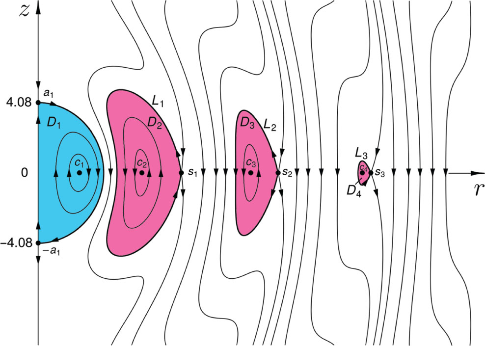
![Figure 2: Poloidal contours of magnetic surfaces Φ1(r,z)=const${\Phi_{1}}(r,z)={\text{const}}$ for the up-down asymmetric plasma equilibrium with flux function Φ1(r,z)=r2[0.0075−zG3(R)]${\Phi_{1}}(r,z)={r^{2}}[0.0075-z{G_{3}}(R)]$ (19). Rotation of the contours around the axis z defines three maximal magnetic rings (pink) and three magnetic blobs (blue).](/document/doi/10.1515/zna-2018-0337/asset/graphic/j_zna-2018-0337_fig_002.jpg)
![Figure 9: Plots of functions y1(u)=G2(u)${y_{1}}(u)={G_{2}}(u)$ and y2(u)=−[G1(u)+G2(u)]/2${y_{2}}(u)=-[{G_{1}}(u)+{G_{2}}(u)]/2$.](/document/doi/10.1515/zna-2018-0337/asset/graphic/j_zna-2018-0337_fig_009.jpg)