Constructing Quasi-Periodic Wave Solutions of Differential-Difference Equation by Hirota Bilinear Method

1 Introduction

Recently, differential-difference equations have stimulated considerable interest due to their numerous applications in the areas of physics and engineering [1], [2], [3], [4], [5], [6], [7], [8]. Usually, for better understanding of the meaning of differential-difference equations, it is of great significance to search for their exact analytic solutions. The exact solution, if available, of these equations facilitates the verification of numerical solvers and aids in the stability analysis of solutions. In the past decades, there has been significant progression in the development of the methods for exact solutions such as inverse scattering method [9], Darboux transformation [10], [11], Hirota bilinear method [12], [13], algebro-geometric method [14], [15], [16], [17], [18], [19], and others.

Among them, the algebro-geometric method is an analogue of inverse scattering transformation, which was first developed by Matveev, Its, Novikov, and Dubrovin et al. The method can derive an important class of exact solutions, which is called algebro-geometric or quasi-periodic solution, to many soliton equations such as Korteweg-de Vries (KdV) equation, sine-Gordon equation, and Schrödinger equation. In recent years, such solutions of nonlinear equations have aroused much interest in mathematical physics [20], [21], [22], [23], [24], [25]. However, this method usually is applied in the integrable nonlinear evolution equations admitting Lax pairs representation and involves complicated algebraic geometry theory which often requires the use of Riemann theta functions and calculus on Riemann surfaces [26], [27], [28]. These have been used far less than their soliton counterparts.

It is well known that the bilinear derivative method developed by Hirota is a powerful and direct approach to construct the exact solution of nonlinear equations [12], [13], [29], [30], [31], [32], [33], [34], [35]. Once a nonlinear equation is written in bilinear form by a dependent variable transformation, then multi-soliton solutions and rational solutions can be obtained. Recently, by means of the Hirota bilinear method, Nakamura proposed a convenient way to construct quasi-periodic solutions of nonlinear equation in his two serial papers [36], [37], where the periodic wave solutions of the KdV equation and the Boussinesq equation were obtained. Some authors, such as Ma, Zhang, Fan, and their collaborators have extended this method to investigate the breaking soliton equation, the Boussinesq equation, KdV, Kadomtsev–Petviashvili, asymmetric Nizhnik-Novikov-Vesselov, and Bogoyavlenskii equations [38], [39], [40], [41], [42]. In fact, the appeal and success of this method lies in the fact that it circumvents complicated algebro-geometric theory to directly get explicit quasi-periodic wave solutions. And this method also shows its effectiveness to some special types of equations, e.g. supersymmetric equations [43], [44]. However, little work has been done on differential-difference equations for the quasi-periodic wave solutions by using the Hirota bilinear method [45], [46], and it is shown that all parameters appearing in the quasi-periodic wave solutions are conditionally free variables, whereas usual quasi-periodic solutions involve some Riemann constants which are difficult to be determined explicitly.

In the present paper, based on the Riemann theta function, we extend the Hirota bilinear method to directly construct quasi-periodic solutions for the differential-difference equations. A new integrable generalized differential-difference equation [47] is taken as an example to illustrate the method. It will be shown that its soliton solution can be obtained as a limiting case of the quasi-periodic wave solution under certain conditions and small amplitude limit.

The rest of the paper is organized as follows. In Section 2, we briefly recall bilinear form of differential-difference equation and the Riemann theta function. In Section 3, we apply the Hirota bilinear method and Riemann theta function to construct quasi-periodic wave solutions to a differential-difference equation. Further, we analyze the asymptotic behavior of the quasi-periodic wave solutions in detail in the last section. It is rigorously shown that a well-known soliton solution can be obtained from the quasi-period wave solution under a “small amplitude” limit. Further work about the multi-periodic wave solutions of differential-difference equations will be given in final.

2 The Bilinear Form and the Riemann Theta Function

In this section, we first briefly recall the integrable generalized differential-difference equation [47] whose bilinear form is

where k₁ and k₂ are two integers, α is an arbitrary constant, and c is an integration constant. The bilinear differential operator D_t and difference operator eDn are defined by

Bilinear form (1) covers many famous differential-difference equations. In particular, when k₁=1, k₂=2, (1) can easily transform into the generalized Lotka-Volterra equation found by Tsujimoto and Hirota [48]; when α=0, taking the transformation

the famous extended Lotka-Volterra equation [49], [50]

can be recovered. As shown in [47] (1) is integrable in the sense of Bäcklund transformation.

The operators D_t, eDn, and sinh(δD_n) have very good properties when they act on exponential functions

where ξ_j=ω_jt+ν_jn+σ_j, j=1, 2. More generally, we have

G(Dt, sinh(δDn))eξ1⋅eξ2=G(ω1−ω2, sinh(δ(ν1−ν2)))eξ1 + ξ2

where G(D_t, sinh(δD_n)) is a polynomial function with respect to the operators D_t and sinh(δD_n).

In the special case of c=0, (1) admits one-soliton solution

In the following, we introduce a one-dimensional Riemann theta function and discuss its quasi-periodicity, which plays a central role in this paper. The Riemann theta function reads

Here the integer value m∈ℤ, s, ϵ∈ℂ, and complex phase variables ξ=ωt+νn+σ is dependent on continuous time variable t and discretized spacial variable n. The τ>0 is called the period matrix of the Riemann theta function. For simplicity, in the case when s=ϵ=0, we denote

Definition 2.1. A function g(t) on ℂ is said to be quasi-periodic in t with fundamental periods T₁, …, T_k∈ℂ if T₁, …, T_k are linearly dependent on ℤ, and there exists a function G(y₁, …, y_k)∈ℂ_k, such that

for all (y₁, …, y_k)∈ℂ_k,

In particular, g(t) becomes periodic with the period T if and only if T_j=m_jT.

Proposition 2.2. The Riemann theta function ϑ(ξ, τ) defined above has the periodic properties [51], [52]

Proposition 2.3. The meromorphic functions F(ξ) on ℂ are as follows:

Then all three cases (i)–(iii) hold that

that is, these F(ξ) are quasi-periodic functions with two fundamental periods 1 and iτ [46].

3 The Quasi-Periodic Solution

Now we consider the Riemann theta function solution of the above bilinear form differential-difference equation (1)

where m∈ℤ, τ>0, and ξ=ωt+νn+σ.

Substituting (14) into (1) gives

Let m′=h+l, and using the relations

we finally obtain that

where

It is seen that if the following equations C(ω, ν, μ)=0 are satisfied, for all possible combinations μ=0, 1, then ϑ(ξ, τ) is a solution of the bilinear equation (1). On the other hand, the equations G(ω, ν, 0)=0 and G(ω, ν, 1)=0 can be explicitly written as

i.e.

where by convention the prime means ∂ξ and

By introducing the notations

systems (21) and (22) admit an explicit solution

Finally, we can obtain the quasi-periodic solution for the differential-difference equation (1)

where ξ=ωt+νn+σ, ν and σ are arbitrary constants, and ω and c are given by (25).

4 Asymptotic Property

In the following, we further consider asymptotic property of the one-periodic wave solution. We will directly use system (25) to analyze the asymptotic properties of the periodic solution. It will be shown that the one-soliton solution can be obtained as a limiting case of the one-periodic wave solution (26). The relations between these two solutions are established as follows.

Theorem 4.1. Suppose that the vector (ω, c) is a solution of system (25), and for the periodic wave solution (25), we let

where the ν and σ are arbitrary constants. Then we have the following asymptotic properties

η=ν′n+2sinh(k2ν′2)[(1−α)sinh(ν′k12)cosh(ν′k22)−(1+α)cosh(ν′k12)sinh(ν′k22)]sinh(k1ν′2)t+σ′,θ(ξ, τ)→1+eη,   as   λ→0.

In other words, the periodic solution (25) tends to the soliton solution (6) under a small amplitude limit.

Proof. Here we will directly use system (25) to analyze the asymptotic properties of periodic solution, which is more simple and effective than the original method of solving system (25) as done in [40], [41]. Since the coefficients of system (24) are power series about λ, its solution (ω, c) also should be a series about λ. We explicitly expand the coefficients of system (24) as follows

Let the solution of system (25) be in the form

Substituting the expansions (29) and (30) into system (25) and letting λ→0, we immediately obtain the following relations

Combining (30) and (31) leads to

or equivalently,

It remains to consider asymptotic property of the one-periodic wave solution (26) under the limit λ→0. For this purpose, we expand the Riemann theta function ϑ(ξ, τ) and make use of expression (33); it follows that

which proves the above theorem. Therefore, we conclude that the periodic solution (26) just goes to the soliton solution (6) as the amplitude λ→0.         □

As illustrated at the beginning of Section 2, the bilinear form (1) is so general that it covers many famous differential-difference equations. For example, taking the transformation of solution (3), the extended Lotka-Volterra equation (4) becomes the bilinear form (1) with α=0 [50]. Then by the above analysis, we can directly get the quasi-periodic solution a_n of the extended Lotka-Volterra equation (4). The quasi-periodic and the corresponding soliton solutions of the extended Lotka-Volterra equation have been presented in Figures 1 and 2.

Figure 1:

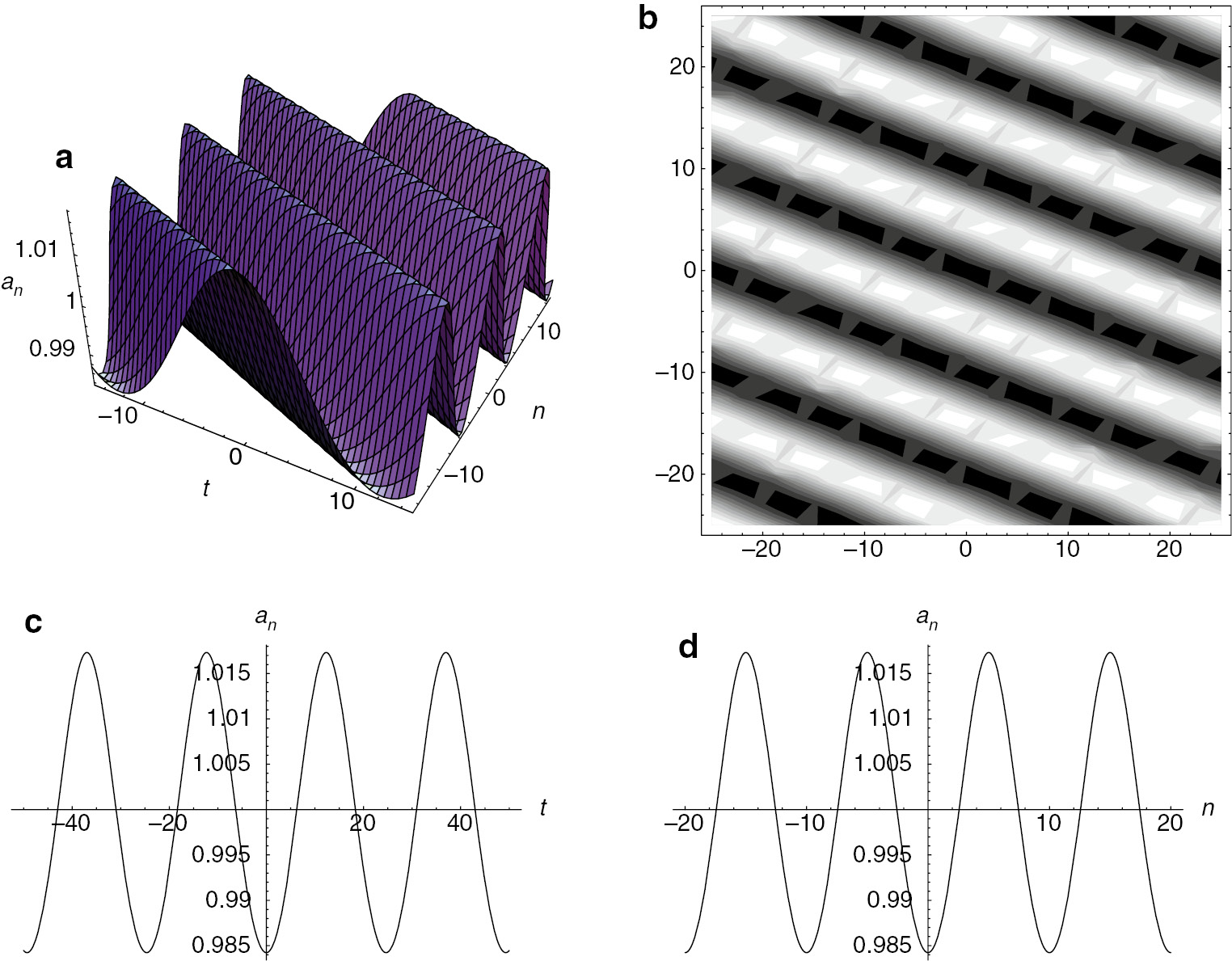
Quasi-periodic wave for the extended Lotka-Volterra equation (4): (a) perspective view of wave, (b) overhead view of wave, with contour plot shown, (c) along t-axis, and (d) along n-axis, where ν=0.1, k₁=2, k₂=1, σ=0 and τ=1.

Figure 2:

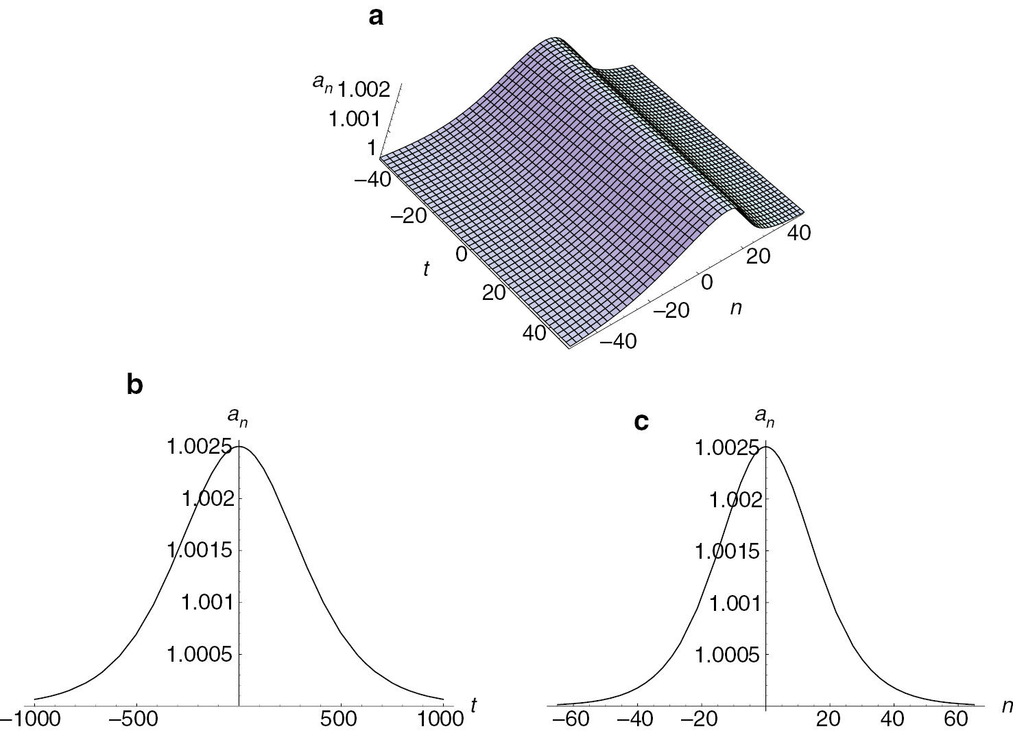
Solitary wave for the extended Lotka-Volterra equation (4): (a) perspective view of wave, (b) along t-axis, and (c) along n-axis, where ν=0.1, k₁=2, k₂=1, σ=0 and τ=1.

5 Multi-Periodic Wave Solutions

Following the procedure described in this paper, we are able to construct quasi-periodic wave solutions for other differential-difference equations. Moveover, we can construct multi-periodic wave solutions of differential-difference equations by the multi-dimensional Riemann theta function as the following form

where ξ=(ξ₁, ξ₂, …, ξ_N)^T∈ℂ_N, m=(m₁, m₂, …, m_N)_T∈ℤ_N, ξ_j=ω_jt+ν_jn+σ_j, j=1, …, N, τ is a N×N symmetric positive definite matrix. The inner product is defined by

for two vectors f=(f₁, f₂, …, f_N)_T and g=(g₁, g₂, …, g_N)_T.

To make the multi-dimensional Riemann theta function (35) satisfy the bilinear equation (1), from (18) we have

It is very important to consider the number of equations and unknown parameters. Obviously, in the case of differential-difference equations, the number of constraint equations of the type (17) is 2_N. On the other hand, we have parameters τ_jk=τ_kj, ω_j, ν_j, and c whose total number is 12N(N+1)+2N+1. Among them, 2N parameters τ_jj and ν_j are taken to be the given parameters related to the amplitudes and wave numbers (or frequencies) of N-periodic waves. 12N(N−1) parameters τ_jk implicitly appear in series form, which in general cannot to be solved explicitly. Hence, the number of explicit unknown parameters is only N+1. The number of equations is larger than the unknown parameters in the case when N≥2. In this paper, we consider one-periodic wave solution of (1), which belongs to the case when N=1. There are still certain difficulties in the calculation for the case N≥2, which will be considered in our future work.

References

[1] E. Fermi, J. Pasta, and S. Ulam, Collected Papers of Enrico Fermi II, University of of Chicago Press, Chicago 1965.Suche in Google Scholar
[2] M. Wadati and M. Toda, J. Phys. Soc. Jpn. 39, 1196 (1975).10.1143/JPSJ.39.1196Suche in Google Scholar
[3] D. Levi and O. Ragnisco, Lett. Nuovo Cimento 22, 691 (1978).10.1007/BF02813707Suche in Google Scholar
[4] S. I. Svinolupov and R. I. Yamilov, Phys. Lett. A 160, 548 (1991).10.1016/0375-9601(91)91066-MSuche in Google Scholar
[5] R. I. Yamilov, J. Phys. A: Math. Theor. 27, 6839 (1994).10.1088/0305-4470/27/20/020Suche in Google Scholar
[6] V. E. Adler, S. I. Svinolupov, and R. I. Yamilov, Phys. Lett. A 254, 24 (1999).10.1016/S0375-9601(99)00087-0Suche in Google Scholar
[7] A. B. Shabat and R. I. Yamilov, Leningrad Math. J. 2, 377 (1991).Suche in Google Scholar
[8] E. G. Fan and H. H. Dai, Phys. Lett. A 372, 4578 (2008).10.1016/j.physleta.2008.04.051Suche in Google Scholar
[9] M. J. Ablowitz and P. A. Clarkson, Solitons, Nonlinear Evolution Equations and Inverse Scattering, Cambridge University Press, New York 1991.10.1017/CBO9780511623998Suche in Google Scholar
[10] V. B. Matveev and M. A. Salle, Darboux Transformation and Solitons, Springer, Berlin 1991.10.1007/978-3-662-00922-2Suche in Google Scholar
[11] C. H. Gu, H. S. Hu, and Z. X. Zhou, Darboux Transformations in Soliton Theory and Its Geometric Applications, Shanghai Science Technology Publisher, Shanghai 1999.Suche in Google Scholar
[12] R. Hirota and J. Satsuma, Prog. Theor. Phys. 57, 797 (1977).10.1143/PTP.57.797Suche in Google Scholar
[13] R. Hirota, The Direct Methods in Soliton Theory, Springer-Verlag, Berlin 2004.10.1017/CBO9780511543043Suche in Google Scholar
[14] B. A. Dubrovin, Funct. Anal. Appl. 9, 41 (1975).10.1007/BF01078183Suche in Google Scholar
[15] A. Its and V. Matveev, Funct. Anal. Appl. 9, 69 (1975).10.1007/BF01078185Suche in Google Scholar
[16] E. Belokolos, A. Bobenko, V. Enol’skij, A. Its, and V. Matveev, Algebro-Geometrical Approach to Nonlinear Integrable Equations, Springer, Berlin 1994.Suche in Google Scholar
[17] S. P. Novikov, S. V. Manakov, L. P. Pitaeskii, and V. E. Zakharov, Theory of Solitons, The Inverse Scattering Methods, Nauka, Moscow 1980.Suche in Google Scholar
[18] P. L. Christiansen, J. C. Eilbeck, V. Z. Enolskii, and N. A. Kostov, Proc. R. Soc. London A Math. 451, 685 (1995).10.1098/rspa.1995.0149Suche in Google Scholar
[19] R. G. Zhou, J. Math. Phys. 38, 2535 (1997).10.1063/1.531993Suche in Google Scholar
[20] C. W. Cao, Y. T. Wu, and X. G. Geng, J. Math. Phys. 40, 3948 (1999).10.1063/1.532936Suche in Google Scholar
[21] X. G. Geng and Y. T. Wu, J. Math. Phys. 40, 2971 (1999).10.1063/1.532739Suche in Google Scholar
[22] X. G. Geng, C. W. Cao, and H. H. Dai, J. Phys. A: Math. Theor. 34, 989 (2001).10.1088/0305-4470/34/5/305Suche in Google Scholar
[23] Z. J. Qiao, Rev. Math. Phys. 13, 545 (2001).10.1142/S0129055X01000752Suche in Google Scholar
[24] C. W. Cao, X. G. Geng, and H. Y. Wang, J. Math. Phys. 43, 621 (2002).10.1063/1.1415427Suche in Google Scholar
[25] H. H. Dai and X. G. Geng, Chaos Soliton. Fract. 18, 1031 (2003).10.1016/S0960-0779(03)00061-4Suche in Google Scholar
[26] E. D. Belokolos, A. I. Bobenko, V. Z. Enol’Skii, and A. R. Its, Algebro-Geometric Approach to Nonlinear Integrable Equations, Springer-Verlag, Berlin 1994.Suche in Google Scholar
[27] B. A. Dubrovin, Russ. Math. Surv. 36, 11 (1981).10.1070/RM1981v036n02ABEH002596Suche in Google Scholar
[28] I. M. Krichever, Acta Appl. Math. 36, 7 (1994).10.1007/BF01001540Suche in Google Scholar
[29] X. B. Hu and P. A. Clarkson, J. Phys. A: Math. Theor. 28, 5009 (1995).10.1088/0305-4470/28/17/029Suche in Google Scholar
[30] X. B. Hu, C. X. Li, J. J. C. Nimmo, and G. F. Yu, J. Phys. A: Math. Theor. 38, 195 (2005).10.1088/0305-4470/38/1/014Suche in Google Scholar
[31] R. Hirota and Y. Ohta, J. Phys. Soc. Jpn. 60, 798 (1991).10.1143/JPSJ.60.798Suche in Google Scholar
[32] D. J. Zhang, J. Phys. Soc. Jpn. 71, 2649 (2002).10.1143/JPSJ.71.2649Suche in Google Scholar
[33] W. X. Ma, Mod. Phys. Lett. B 19, 1815 (2008).10.1142/S0217984908016492Suche in Google Scholar
[34] K. Sawada and T. Kotera, Prog. Theor. Phys. 51, 1355 (1974).10.1143/PTP.51.1355Suche in Google Scholar
[35] Y. Ohta, K. I. Maruno, and B. F. Feng, J. Phys. A: Math. Theor. 41, 355205 (2008).10.1088/1751-8113/41/35/355205Suche in Google Scholar
[36] A. Nakamura, J. Phys. Soc. Jpn. 47, 1701 (1979).10.1143/JPSJ.47.1701Suche in Google Scholar
[37] A. Nakamura, J. Phys. Soc. Jpn. 48, 1365 (1980).10.1143/JPSJ.48.1365Suche in Google Scholar
[38] H. H. Dai, E. G. Fan, and X. G. Geng, Available at: http://arxiv.org/pdf/nlin/0602015.Suche in Google Scholar
[39] W. X. Ma, R. G. Zhou, and L. Gao, Mod. Phys. Lett. A 24, 1677 (2009).10.1142/S0217732309030096Suche in Google Scholar
[40] Y. Zhang, L. Y. Ye, Y. N. Lv, and H. Q. Zhao, J. Phys. A: Math. Theor. 40, 5539 (2007).10.1088/1751-8113/40/21/006Suche in Google Scholar
[41] E. G. Fan, J. Phys. A: Math. Theor. 42, 095206 (2009).10.1088/1751-8113/42/9/095206Suche in Google Scholar
[42] E. G. Fan and Y. C. Hon, Phys. Rev. E 78, 036607 (2008).10.1103/PhysRevE.78.036607Suche in Google Scholar PubMed
[43] E. G. Fan and Y. C. Hon, Stud. Appl. Math. 125, 343 (2010).10.1111/j.1467-9590.2010.00491.xSuche in Google Scholar
[44] Y. C. Hon and E. G. Fan, Theor. Math. Phys. 166, 317 (2011).10.1007/s11232-011-0026-xSuche in Google Scholar
[45] Y. C. Hon, E. G. Fan, and Z. Y. Qin, Mod. Phys. Lett. B 22, 547 (2008).10.1142/S0217984908015097Suche in Google Scholar
[46] E. G. Fan and K. W. Chow, Phys. Lett. A 374, 3629 (2010).10.1016/j.physleta.2010.07.005Suche in Google Scholar
[47] X. B. Hu, P. A. Clarkson, and R. Bulloughx, J. Phys. A: Math. Theor. 30, L669 (1997).10.1088/0305-4470/30/20/002Suche in Google Scholar
[48] S. Tsujimoto and R. Hirota, J. Phys. Soc. Jpn. 65, 2797 (1996).10.1143/JPSJ.65.2797Suche in Google Scholar
[49] K. Narita, J. Phys. Soc. Jpn. 51, 1682 (1982).10.1143/JPSJ.51.1682Suche in Google Scholar
[50] X. B. Hu and P. A. Clarkson, J. Nonlinear Math. Phys. 9, 75 (2002).10.2991/jnmp.2002.9.s1.7Suche in Google Scholar
[51] H. M. Farkas and I. Kra, Riemann Surfaces, Springer-Verlag, New York 1992.10.1007/978-1-4612-2034-3Suche in Google Scholar
[52] D. Mumford, Theta Lectures on Theta II, Birkhäuser, Boston 1983.10.1007/978-1-4899-2843-6Suche in Google Scholar
©2016 Walter de Gruyter GmbH, Berlin/Boston
Artikel in diesem Heft
- Frontmatter
- Oscillations in the Interactions Among Multiple Solitons in an Optical Fibre
- The Successive Application of the Gauge Transformation for the Modified Semidiscrete KP Hierarchy
- A Steady-state Trio for Bretherton Equation
- Convective Fins Problem with Variable Thermal Conductivity: An Approach Based on Embedding Green’s Functions into Fixed Point Iterative Schemes
- Liouville Correspondence Between the Short-Pulse Hierarchy and the Sine-Gordon Hierarchy
- The Effect of Variable Viscosities on Micropolar Flow of Two Nanofluids
- Soliton and Shock Profiles in Electron-positron-ion Degenerate Plasmas for Both Nonrelativistic and Ultra-Relativistic Limits
- Lump Solutions for the (3+1)-Dimensional Kadomtsev–Petviashvili Equation
- Sudden and Slow Quenches into the Antiferromagnetic Phase of Ultracold Fermions
- A Discrete Negative Order Potential Korteweg–de Vries Equation