A Note on Exact Solutions for the Unsteady Free Convection Flow of a Jeffrey Fluid

1 Introduction

Fluids that obey Newton’s law of viscosity are known as Newtonian fluids. These fluids make the simplest mathematical models of fluids that account for viscosity. Examples of Newtonian fluids include air, water, ethanol, benzene and mineral oils. However, many materials encountered in industry and medicine that fall outside the group of classical models of Newtonian fluids are known as non-Newtonian fluids. All high-viscosity liquids as well as polymer solutions, molten polymers, many solid suspensions, blood, colloids, gels, concentrated slurries and the solutions of macromolecules exhibit non-Newtonian behaviour [1].

The study of non-Newtonian fluids has not progressed far enough to develop many useful theoretical approaches. Of course, it is due to the diversity of non-Newtonian fluids in nature. Hence, no unique relationship is available in the literature that can describe the rheology of all non-Newtonian fluids and various types of these fluids exist. Further, the partial differential equations governing the flow of non-Newtonian fluids are of higher order and complicated in comparison to those governing the flow of Newtonian fluids [2–4].

Amongst the variety of rheological models proposed to represent non-Newtonian fluids, the one that is most widely used is the Jeffrey model. This fluid model is a relatively simpler linear model that uses time derivatives instead of convected derivatives the same way as the Oldroyd-B model does. But a careful study of the literature shows that the Jeffrey model has received very little attention. Keeping these facts in mind, we have chosen this model for the present analysis. Khadrawi et al. [5] obtained semi-analytical solutions for three basic viscoelastic fluid flow problems under the effect of the Jeffrey model. The Laplace transform technique is used for finding the solutions. However, it is not always easy to find the inverse Laplace transform. Therefore, they inverted the transform solutions using the Riemann sum approximation. Khan et al. [6] investigated some unsteady flows of a Jeffrey fluid between two side walls perpendicular to a plate and established exact solutions using integral transforms. Mekheimer et al. [7] performed Lie group analysis and studied the two-dimensional boundary layer flow of an electrically conducting Jeffrey fluid. Siddiqui et al. [8] studied the classical Von Karman flow problem for a Jeffrey fluid by using a generalized non-similarity transformation. Ali and Asghar [9] reported the study of two-dimensional oscillatory flow inside a rectangular channel for a Jeffrey fluid with small suction. Few other attempts for the Jeffrey fluid can also be found in [10–15].

On one hand heat transfer due to free convection has been studied most extensively because of its frequent use in nature as well as in engineering and environmental applications such as in nuclear power plants and in chemical reactors (see [16–18] and the references therein). On the other hand such studies for Jeffrey fluid are very rare. Keeping in mind the importance of the free convection flow of a Jeffrey fluid, Kavita et al. [19] analysed the influence of heat transfer on the magnetohydrodynamic (MHD) oscillatory flow of a Jeffrey fluid in a channel. They used the constitutive equations of a Jeffrey fluid and derived the unsteady governing equations of momentum and energy under the Boussinesq approximation. We have found that the momentum equation (2.2) in their paper is missing the third-order term multiple of the retardation parameter. Hence they found some erroneous results given by (3.10). In another paper [20], the same authors studied the effects of a magnetic field on the free convective flow of a Jeffrey fluid past an infinite vertical porous plate with constant heat flux. A perturbation series solution was used to obtain the velocity field and temperature field for small values of the Eckert number. However, due to the assumption of steady motion, the third-order term of velocity in the momentum equation automatically vanishes.

The aim of this short note is twofold: first, to model and use the correct form of the governing equations for a Jeffrey fluid, and second, to find the exact solutions. This is because in most of the above studies on a Jeffrey fluid, the solutions are obtained either in numerical form or by using any approximate method. Therefore, it is important to carry out a study on unsteady free convection flow of a Jeffrey fluid with exact solutions. Exact solutions, on the other hand, are important for many reasons. They provide a standard for checking the accuracies of many approximate methods such as numerical or asymptotic. Also, these solutions can be used as a benchmark by numerical solvers and experimentalists for checking the stability of their solutions. Therefore, in the present paper, an exact analysis is carried out to investigate the heat transfer analysis due to free convection of a Jeffrey fluid over a vertical plate. The Laplace transform technique is used for finding the exact solutions.

2 Mathematical Formulation

The constitutive equations for a Jeffrey fluid are given by

(1)T = −pI + S, (1)

(2)S = μ1 + λ1[A1 + λ2dA1dt]; ddt = ∂∂t + V⋅∇, (2)

where −pI is the indeterminate part of the stress, S is the extra stress tensor, μ is the coefficient of viscosity and λ₁ and λ₂ are the material parameters of a Jeffrey fluid. It is remarkable here to mention that for λ₁=λ₂=0, this model reduces to the classical viscous Newtonian fluid.

The Rivlin–Ericksen tensor A₁ is defined as

(3)A1 = L + LT; L = ∇V. (3)

Now let us consider the unsteady free convection flow of a Jeffrey fluid near an isothermal vertical plate situated in the (x, z) plane of a Cartesian coordinate system x, y and z. Initially, both the plate and fluid are at rest at a constant temperature T_∞. At time t=0⁺, the temperature of the plate rises to T_w and thereafter remains constant. For unidirectional and one-dimensional flow velocity, temperature and stress fields are

(4)v = v(y; t) = u(y, t)i; S = S(y; t); T = T(y, t), (4)

where i is the unit vector along the x-direction of the Cartesian coordinate system and the stress field satisfies the condition S(y; 0)=0. We obtain S_xx=S_yy=S_zz=S_xz=S_zx=S_yz=S_zy=0 and

(5)Sxy = μ1 + λ1(1 + λ2∂∂t)∂u∂y, (5)

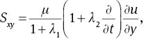
where S_xy is the non-trivial tangential stress.

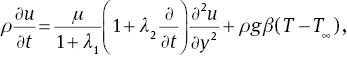
Under the above assumptions and using (4)₁, the continuity equation satisfies identically. Using (1)–(5) and the Boussinesq approximation, the equations of momentum and energy for the free convection flow of an incompressible Jeffrey fluid are given by

(6)ρ∂u∂t = μ1 + λ1(1 + λ2∂∂t)∂2u∂y2 + ρgβ(T − T∞), (6)

(7)∂T∂t = kρcp∂2T∂y2. (7)

The corresponding initial and boundary conditions are

(8)u(y, 0) = 0, T(y, 0) = T∞, y > 0,u(0, t) = 0, T(0, t) = Tw, t > 0,u(∞, t) = 0, T(∞, t) = T∞, t > 0. (8)

In the above equations [(6)–(8)], u=u(y, t) denotes the fluid velocity in the x-direction, T=T(y, t) is the temperature, ρ is the constant density of the fluid, g is the acceleration due to gravity, c_p is the specific heat capacity, k is the thermal conductivity, T_w is the wall temperature and T_∞ is the free stream temperature.

Introducing the non-dimensional variables

(9)u′ = uu0, y′ = yu0ν, t′ = tu02ν, θ = T − T∞Tw − T∞, τ = Sxyνμu02, (9)

into (5)–(8), we get (prime notations are dropped for simplicity)

(10)∂u∂t = 11 + λ1(1 + λ∂∂t)∂2u∂y2 + Grθ, (10)

(11)τ = 11 + λ1(1 + λ∂∂t)∂u∂y, (11)

(12)Pr∂θ∂t = ∂2θ∂y2, (12)

(13)u(y, 0) = 0, θ(y, 0) = 0, y > 0, (13)

u(0, t) = 0, θ(0, t) = 1, t > 0,

(14)u(∞, t) = 0, θ(∞, t) = 0, t > 0, (14)

where

λ = λ2u02ν, Gr = gβν(Tw − T∞)u03 (Grashof number),Pr = μCPk (Prandtl number).

3 Solution of the Problem

In order to determine the exact solutions to the problem defined by (10)–(13), the Laplace transform technique is used. Consequently, applying Laplace transforms to (10)–(12) and using the initial and boundary conditions (13) and (14), we find that

(15)u¯(y, q) = a1q2(q − a0)exp(−ya2qq + λ0) − a1q2(q − a0)exp(−yPr q), (15)

(16)τ¯(y, q) = −a3q + λ0qq(q − a0)exp(−ya2qq + λ0)+ a4(q + λ0)qq(q − a0)exp(−yPr q), (16)

(17)θ¯(y, q) = 1qexp(−yPr q), (17)

where

λ0 = 1λ2; a0 = 1 + λ1 − PrPrλ2; a1 = Gr(1 + λ1)Prλ2;a2 = 1 + λ1λ2; a3 = a1λa21 + λ1; a4 = a1λPr1 + λ1.

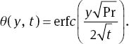
By taking the inverse Laplace transform of (17), one obtains

(18)θ(y, t) = erfc(yPr2t). (18)

In order to find the inverse Laplace of (15), we first arrange it in the following form:

(19)u¯(y, q) = u¯4(y, q) + u¯3(y, q); u¯4(y, q) = u¯1(q)u¯2(y, q), (19)

where

(20)u¯1(q) = (−a1a021q − a1a01q2 + a1a021q − a0),u¯2(y, q) = exp(−ya2qq + λ0), (20)

(21)u¯3(y, q) = (a1a021q + a1a01q2 − a1a021q − a0)exp(−yPr q). (21)

The inverse Laplace transforms of (20)₁ and (21) yield [2]

(22)u1(t) = −a1a02 − a1a0t + a1a02ea0t, (22)

(23)u3(y, t) = a1a02[erfc(yPr2t)]+ a1a0[(t + y2Pr2)erfc(yPr2t)− ytPrπexp(−y2Pr4t)]−a1ea0t2a02[exp(yPra0)erfc(yPr2t + a0t)+ exp(−yPra0)erfc(yPr2t − a0t)]. (23)

In order to determine the function u₂(y, t), we use the inversion formula of compound functions [2, Appendix (A.1)] choosing f(y, q) and w(q) as being given by

(24)f(y, q) = exp(−ya2q) and w(q) = qq + λ0. (24)

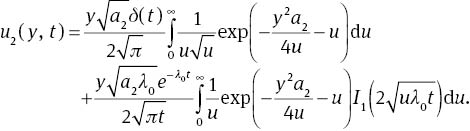
Following [2, see Eqs. (A.2) and (A.3) from Appendix], we immediately obtain

(25)f(y, t) = ya22tπtexp(−y2a24t),g(u, t) = e−u(δ(t) + uλ0te−λ0tI1(2uλ0t)). (25)

Here δ(·) is the Dirac delta function and I₁(·) is the modified Bessel function of the first kind of order 1. Thus

u2(y, t) = ∫0∞f(y, u)g(u, t)du,

and using (25), we get

(26)u2(y, t) = ya2δ(t)2π∫0∞1uuexp(−y2a24u − u)du+ya2λ0e−λ0t2πt∫0∞1uexp(−y2a24u − u)I1(2uλ0t)du. (26)

Inverting (19)₂, we can write u₄(y, t) as a convolution product, i.e.,

(27)u4(y, t) = ∫0tu1(t − s)u2(y, s)ds = ∫0tu1(s)u2(y, t − s)ds. (27)

Incorporating (22) and (26) into (27), we get

(28)u4(y, t) = ya22π(−a1a02 − a1a0t + a1a02ea0t)∫0∞1uuexp(− y2a24u − u)du− ya1a2λ02a02π∫0t∫0∞exp(−y2a24u − u − λ0s)usI1(2uλ0s)du ds− ya1a2λ02a0π∫0t∫0∞exp(−y2a24u − u − λ0s)usI1(2uλ0s)(t − s)du ds+ ya1a2λ0ea0t2a02π∫0t∫0∞exp(−y2a24u − u − a0s − λ0s)usI1(2uλ0s)du ds. (28)

Using the relation from Appendix (A.4) from [2], we can write

(29)∫0∞1uuexp(−y2a24u − u)du = 2πe−a2ya2y. (29)

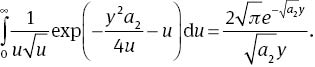
Substituting (29) into (28), we get

(30)u4(y, t) = (−a1a02 − a1a0t + a1a02ea0t)exp(−a2y)−ya1a2λ02a02π∫0t∫0∞exp(−y2a24u − u − λ0s)usI1(2uλ0s)du ds−ya1a2λ02a0π∫0t∫0∞exp(−y2a24u − u − λ0s)usI1(2uλ0s)(t − s)du ds+ya1a2λ0ea0t2a02π∫0t∫0∞exp(−y2a24u − u − a0s − λ0s)usI1(2uλ0s)du ds. (30)

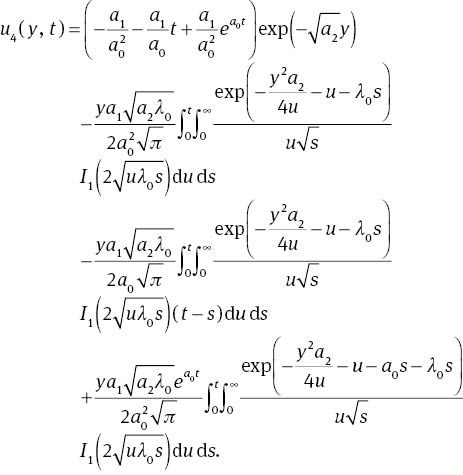
Thus, finally, the inverse Laplace transform of (19) is given by

(31)u(y, t) = u4(y, t) + u3(y, t), (31)

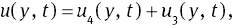
where u₃(y, t) and u₄(y, t) are given by (23) and (30), respectively.

Now to determine the shear stress, we follow the same procedure as in [2], and write

(32)τ(y, t) = τ1(y, t) + τ2(y, t) + τ3(y, t), (32)

where

(33)τ1(y, t) = a4ea0tπ∫0texp(−y2Pr4s − a0s)sds, (33)

(34)τ2(y, t) = 2a4λ0ea0tπ∫0tsexp(−y2Pr4s − a0s)ds− a4λ0yPrea0t∫0te−a0serfc(yPr2s)ds. (34)

(35)τ3(y, t) = a3a0(1 − ea0t)exp(−ya2) + a3λ0a0π∫0t∫0∞1sexp(−y2a24u − u − λ0s)×I1(2uλ0s)du ds − a3λ0ea0ta0π∫0t∫0∞1sexp(−y2a24u − u − (λ0 + a0)s)×I1(2uλ0s)du ds. (35)

4 Conclusions

Exact solutions for the unsteady free convection flow of an incompressible Jeffrey fluid past an isothermal vertical plate are obtained using the Laplace transform method. Expressions for velocity, shear stress and temperature are obtained in closed form. It is found that the obtained solutions satisfy the imposed initial and boundary conditions and can be easily reduced to the similar solutions for Newtonian fluid.

References

[1] R. P. Chabra and J. F. Richardson, Non-Newtonian Flow and Applied Rheology: Engineering Applications, Butterworth-Heinemann, (2nd ed.), 2008.Suche in Google Scholar
[2] M. Nazar, C. Fetecau, D. Vieru, and C. Fetecau, Nonlinear Anal.: Real World Appl. 11, 584 (2010).10.1016/j.nonrwa.2008.10.055Suche in Google Scholar
[3] T. B. Chang, A. Mehmood, O. A. Beg, M. Narahari, M. N. Islam, et al. Commun. Nonlinear Sci. Numer. Simul. 16, 216 (2011).10.1016/j.cnsns.2010.02.018Suche in Google Scholar
[4] F. Ali, I. Khan, S. Haq, and S. Sharidan, Z. Naturfors. Sect. A-J. Phys. Sci. 67a, 377 (2012).Suche in Google Scholar
[5] A. F. Khadrawi, M. A. Al-Nim, and A. Othman, Chem. Eng. Sci. 60, 7131 (2005).10.1016/j.ces.2005.07.006Suche in Google Scholar
[6] M. Khan, I. Faiza, and A. Anjum, Z. Naturfors. Sect. A-J. Phys. Sci. 66a, 745 (2011).10.5560/zna.2011-0048Suche in Google Scholar
[7] K. S. Mekheimer, S. Z.-A. Husseny, A. T. Ali, and R. E. Abo-Elkhair, Phys. Scr. 83, 015017 (2011).10.1088/0031-8949/83/01/015017Suche in Google Scholar
[8] A. M. Siddiqui, A. A. Farooq, T. Haroon, and B. S. Babcock, Appl. Math. Sci. 7, 983 (2013).10.12988/ams.2013.13089Suche in Google Scholar
[9] A. Ali and S. Asghar, J. Aerosp. Eng. 27, 644 (2014).10.1061/(ASCE)AS.1943-5525.0000298Suche in Google Scholar
[10] R. Ellahi, S. Ur-Rahman, and S. Nadeem, Z. Naturfors. Sect. A-J. Phys. Sci. 68a, 489 (2013).10.5560/zna.2013-0032Suche in Google Scholar
[11] R. Ellahi, M. Mubashir Bhatti, A. Riaz, and M. Sheikholeslami, J. Porous Media 17, 143 (2014).10.1615/JPorMedia.v17.i2.50Suche in Google Scholar
[12] R. Ellahi, A. Riaz, S. Nadeem, and M. Mushtaq, Appl. Math. Inform. Sci. 7, 1441 (2013).10.12785/amis/070424Suche in Google Scholar
[13] S. Nadeem, A. Riaz, R. Ellahi, and N. S. Akbar, Appl. Nanosci. 4, 613 (2014).10.1007/s13204-013-0238-5Suche in Google Scholar
[14] A. Riaz, S. Nadeem, R. Ellahi, and A. Zeeshan, Appl. Biol. Biomech. 11, 81 (2014).10.1155/2014/901313Suche in Google Scholar
[15] R. Ellahi, S. U. Rahman, and S. Nadeem, Phys. Lett. A 378, 2973 (2014).10.1016/j.physleta.2014.08.002Suche in Google Scholar
[16] M. Narahari and B. K. Dutta, Chem. Eng. Commun. 199, 628 (2012).10.1080/00986445.2011.611058Suche in Google Scholar
[17] M. J. Uddin, W. A. Khan, and A. I. Ismail, PLoS One 7, e49499 (2012).10.1371/journal.pone.0049499Suche in Google Scholar PubMed PubMed Central
[18] C. Fetecau, M. Rana, and C. Fetecau, Z. Naturfors. Sect. A-J. Phys. Sci. 68, 130 (2013).10.5560/zna.2012-0083Suche in Google Scholar
[19] K. Kavita, K. R. Prasad, and B. A. Kumari, Adv. Appl. Sci. Res. 3, 2312 (2012).Suche in Google Scholar
[20] B. A. Kumari, K. R. Prasad, and K. Kavitha, Int. J. Math. Arch. 3, 2240 (2012).Suche in Google Scholar
©2015 by De Gruyter
Artikel in diesem Heft