A Note on the Kirchhoff and Additive Degree-Kirchhoff Indices of Graphs

1 Introduction

Let G= (V, E) be a connected graph. For any two distinct vertices i, j∈V, the resistance distance [1] between them, denoted by Ω_ij, is defined as the net effective resistance between nodes i and j in the electrical network constructed from G when each edge is identified as a unit resistor.

Since the appearance of the concept of resistance distance, some resistance distance-based graph invariants have been defined. Among these invariants, a famous one is the Kirchhoff indexR(G) [1] (or total effective resistance [2], or effective graph resistance [3]), which is defined as the sum of resistance distances between all pairs of vertices of G:

(1)R(G) = ∑{i,j} ⊆ VΩij. (1)

Then, two modifications of the Kirchhoff index have been made to take the degrees of vertices into account. The first one is the multiplicative degree-Kirchhoff indexR*(G) introduced by Chen and Zhang [4] as

(2)R∗(G) = ∑{i,j} ⊆ VdidjΩij, (2)

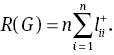
where d_i is the degree (i.e., the number of neighbours) of the vertex i. The second one is the additive degree-Kirchhoff introduced by Gutman et al. [5] as

(3)R+(G) = ∑{i,j} ⊆ V(di + dj)Ωij. (3)

The Kirchhoff index has been widely studied, and we refer the reader to recent papers [6–19] and references therein. However, the study of the additive degree-Kirchhoff index is at an initial stage. In Ref. [5], Gutman et al. characterised n-vertex unicyclic graphs having minimum and second minimum additive degree-Kirchhoff indices. Then, Palacios and his collaborators [20, 21] exhibited various bounds for this index using elegant random walks, majorization, and Schur-convexity techniques. In Refs. [16, 18], the current authors obtained formulae for these Kirchhoffian indices of the subdivision and triangulation of a graph G, which neatly relates their Kirchhoffian indices to that of the original graph G.

In this article, first of all, we establish a relation between the Kirchhoff index and the additive degree-Kirchhoff index by expressing the additive degree-Kirchhoff index in terms of the Kirchhoff index and the Moore–Penrose inverse of the Laplacian matrix of G, so as to yield inequalities for the additive degree-Kirchhoff index via the Kirchhoff index, minimum, maximum, and average degrees. Then, we determine bounds for the Kirchhoff and additive degree-Kirchhoff indices via maximum and minimum degrees, with extremal graphs being characterised. Finally, we obtain an upper bound for the additive degree-Kirchhoff index, which improves the result obtained in Ref. [21].

2 A Relation between the Kirchhoff Index and the Additive Degree-Kirchhoff Index

Let G be a connected graph with n vertices. The adjacency matrixA= (a_ij) of G is the matrix with a_ij=1 if i and j are adjacent and 0 otherwise. Let D=diag{d₁, d₂, …, d_n} be the diagonal matrix of vertex degrees. Then, the Laplacian matrix of G is defined as L=D – A. Because the sum of each row and of each column is zero, L is singular and does not admit an (ordinary) inverse.

Let M be an n×m matrix. Then, the Moore–Penrose inverse of M, denoted by M⁺, is [22] an m×n matrix satisfying the equations:

MM+M = M, M+MM+ = M+, (MM+)H = MM+, (M+M)H = M+M,

where M^H denotes the conjugate transpose of M. It is well known [22] that the Moore–Penrose inverse of a matrix exists and is unique. Let L+ = (lij+) be the Moore–Penrose inverse of L. It is shown that L⁺ plays an essential role in the computation of resistance distance and the Kirchhoff index.

Theorem 1 [1] The resistance distance between vertices i and j can be computed as

(4)Ωij = lii+ + lii+ − 2lij+. (4)

Theorem 2 [23, 24] Let G be a connected graph with n vertices. Then,

(5)R(G) = n∑i = 1n lii+. (5)

Using Theorems 1 and 2, a formula for the additive degree-Kirchhoff index is obtained.

Theorem 3Let G be a connected graph with n vertices and m edges. Then,

(6)R+(G) = 2mnR(G) + n∑i = 1n dilii+ (6)

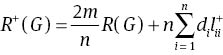
Proof. By the definition of the additive degree-Kirchhoff index, we have

(7)R+(G) = 12∑i = 1n∑j = 1n(di + dj)Ωij= 12∑i = 1n∑j = 1n(di + dj)(lii+ + ljj+ − 2lij+)= 12∑i = 1n∑j = 1n[dilii+ + djljj+ + diljj+ + djlii+ − 2(dilij+ + djlij+)]= 12∑i = 1n∑j = 1n(dilii+ + djljj+) + 12∑i = 1n∑j = 1n(diljj+ + djlii+) − ∑i = 1n∑j = 1n(dilij+ + djlij+)= n∑i = 1n dilii+ + ∑i = 1n di∑j = 1n ljj+ − ∑i = 1n∑j = 1n(dilij+ + djlij+). (7)

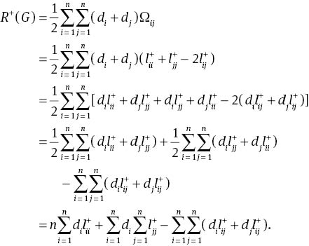
By the fact that ∑i = 1n di = 2m and n∑j = 1n ljj+ = R(G), it follows that

(8)∑i = 1n di∑j = 1n ljj+ = 2mnR(G). (8)

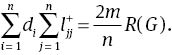
On the other hand, by the fact that L⁺ is symmetric and that the n–vector 1 with all entries equal to 1 is a 0-eigenvalue eigenvector of L⁺, that is, L⁺1=0, we have

(9)∑i = 1n∑j = 1n(dilij+ + djlij+) = ∑i = 1n di∑j = 1n lij+ + ∑j = 1n dj∑i = 1n lji+ = 0. (9)

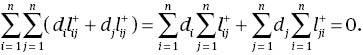
Then, (6) is obtained by substitution of (8) and (9) into (7).

Let δ, Δ, and d̅=(2m/n) denote the minimum, maximum, and average degrees of G, respectively. Then, from the definition of the additive degree-Kirchhoff index, it is obvious that

2δR(G) ≤ R+(G) ≤ 2ΔR(G).

As a consequence of Theorem 3, bounds in the earlier equation can be improved as follows.

Theorem 4R⁺(G) and R(G) satisfy the following inequalities:

(10)(δ + d¯)R(G) ≤ R+(G) ≤ (Δ + d¯)R(G), (10)

with equality if and only if G is d-regular, that is, d= d̅= δ= Δ.

Proof. Noting that d̅=(2m/n) and n∑i = 1nlii+ = R(G), one invokes the inequalities arising upon noting that lii+ ≥ 0 (since L⁺ is non-negative definite) and replacing d_i in Theorem 3 successively by either δ or Δ.       □

3 Bounds for the Kirchhoff and Additive Degree-Kirchhoff Indices via Maximum and Minimum Degrees

We first consider the Kirchhoff index to give an upper bound via the maximum degree as well as a lower bound via the minimum degree. A natural way to bound the Kirchhoff index is first to find the extremal graphs and use their values as bounds. It turns out that T_n,Δ and Knδ as given in the following definitions are extremal graphs.

Definition 1 [25] The broom graph T_n,Δis a tree on n vertices obtained by taking a path P_n-Δ+1and an edgeless graph KΔ − 1¯, and joining one end vertex of the path with every vertex of this edgeless graph.

Definition 2Let Knδ be the graph obtained by taking a complete graph K_n–1and an isolated vertex, and joining δ vertices of K_n–1with the isolated vertex.

For example, graphs T_10,4 and K104 are shown in Figure 1.

Figure 1:

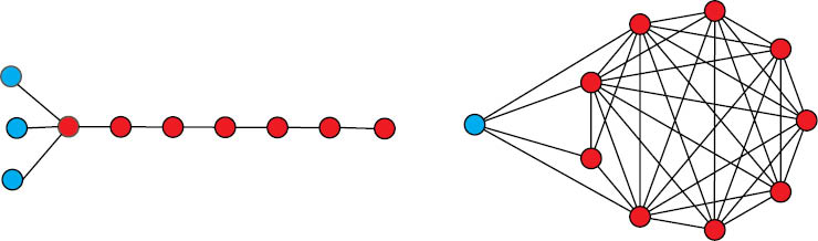
Graphs T_10,4 (left) and K104 (right).

Let 𝒢_n,Δ be the set of all graphs with n vertices and maximum degree Δ. In Refs. [25, 26], it is shown that among all graphs in 𝒢_n,Δ, the graph T_n,Δ has the maximum Wiener index.

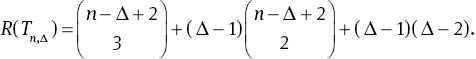
Theorem 5For every graph G∈𝒢_n,Δ,

W(G) ≤ W(Tn,Δ),

with equality if and only if G is isomorphic to T_n,Δ.

Recall [1] that for any graph G, R(G)≤ W(G) with equality if and only if G is a tree. Then, from Theorem 5, for every graph G∈𝒢_n,Δ,

R(G) ≤ W(G) ≤ W(Tn,Δ) ≤ R(Tn,Δ),

with equality if and only if G is isomorphic to T_n,Δ.

Let 𝔾_n,δ be the set of graphs with n vertices and minimum degree δ. Next, we characterise the extremal graph in 𝔾_n,δ with the minimum Kirchhoff index. The following property, known as the non-increasing property of the Kirchhoff index, is used.

Proposition 1 [27] Let G be a connected graph, and let H be a spanning subgraph of G. Then,

R(G) ≤ R(H)

with equality if and only if G ≅ H.

From Proposition 1, it is easily observed as follows.

Lemma 1For every graph G∈𝔾_n,δ,

R(G) ≥ R(Knδ),

with equality if and only if G is isomorphic toKnδ.

Now, we compute Kirchhoff indices for the two extremal graphs T_n,Δ and Knδ. It is shown in Refs. [25, 26] that

(11)R(Tn,Δ) = (n − Δ + 2         3) + (Δ − 1)(n − Δ + 2         2) + (Δ − 1)(Δ − 2). (11)

To compute the Kirchhoff index of Knδ, we first address resistance distances in Knδ. Given a graph G=(V, E), let N(u)={i∈V : iu∈E} and N[u]=N(u)∪{u}.

Lemma 2 [28] Let i and j be vertices of G such that they have the same neighbourhood N in V–{i, j}. Then,

Ωij = {2|N| + 2, if i and j are adjacent, 2|N|, otherwise .

Lemma 3 [29] Let G=(V, E) be a connected graph. Then, for any two vertices, a, b∈V (a ≠ b),

daΩab + ∑i∈N(a)(Ωia − Ωib) = 2.

Theorem 6Let u be the exceptional vertex inKnδ,and letN[u]¯ = V − N[u].Then, resistance distances inKnδare given as

Ωij = {2n, i,j∈ N(u) ,2n − 1, i,j∈ N[u]¯ ,n + δ − 1nδ, i=u and j∈ N(u) ,n + δ(n − 1)δ, i=u and j∈ N[u]¯ ,2nδ − δ + 1n(n − 1)δ, i∈ N(u) and j∈ N[u]¯. 

Proof. If i, j∈N(u), then i and j are adjacent and have the same neighbourhood N=V–{i, j} with |N|=n – 2. Hence, by Lemma 2, it follows that Ω_ij=(2/n). If i,j∈N[u]¯, then again i and j are adjacent and Lemma 2 yields Ω_ij=(2/(n – 1)).

Now, suppose that j∈N(u). To compute Ω_uj, we apply Lemma 3 to u and j, to obtain that

δΩuj + ∑k∈N(u)(Ωuk − Ωjk) = 2.

By symmetry, it is easily seen that for any k∈N(u), Ω_uk=Ω_uj. Thus, the preceding equation becomes

2δΩuj = 2 − ∑k∈N(u)Ωjk = 2 − (δ − 1)2n,

which yields that Ω_uj=((n + δ – 1)/nδ). The case for Ω_uj with j∈N[u]¯ could be obtained in the same way.

Finally, we consider Ω_ij with i∈N(u) and j∈N[u]¯. Again by Lemma 3, we have

djΩji + ∑k∈N(j)(Ωkj − Ωki) = 2,

that is,

(n − 2)Ωji + ∑k∈N(u)(Ωkj − Ωki) + ∑k∈N[u]¯ − j(Ωkj − Ωki) = 2.

By symmetry, the preceding equation becomes

(n − 2)Ωji + δΩij − ∑k∈N(u)Ωki + ∑k∈N[u]¯ − jΩkj − (n − 2 − δ)Ωij = 2.

Simple calculation leads to

2δΩji = 2 + ∑k∈N(u)Ωki − ∑k∈N[u]¯ − jΩkj = 2 + (δ − 1)2n − (n − δ − 2)2n − 1= 4nδ − 2δ + 2n(n − 1).

This gives Ω_ji=(2nδ – δ + 1)/(n(n – 1)δ).

Thus, the proof is complete.         □

As a corollary of Lemma 2, the Kirchhoff index of Knδ is obtained.

Corollary 1

(12)R(Knδ) = n − 1 + nδ − δ + 1n − 1. (12)

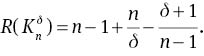
Proof.

R(Knδ) = (δ2)2n + (n − 1 − δ2)2n − 1 + δn + δ − 1nδ + (n − 1 − δ)n + δ(n − 1)δ+ δ(n − 1 − δ)2nδ − δ + 1n(n − 1)δ= δ(δ − 1)n + (n − 1 − δ)(n − 2 − δ)n − 1 + n + δ − 1n + (n + δ)(n − 1 − δ)(n − 1)δ+ (n − 1 − δ)(2nδ − δ + 1)n(n − 1)= n − 1 + nδ − δ + 1n − 1.

Recalling the results in Theorem 5 and Lemma 1, together with (11) and (12), the main result is obtained.

Theorem 7Let G be a n-vertex connected graph with minimum degree δ and maximum degree Δ (Δ≥ 2). Then,

n − 1 + nδ − δ + 1n − 1 ≤ R(G) ≤ (n − Δ + 23) + (Δ − 1)(n − Δ + 22) + (Δ − 1)(Δ − 2).

The first equality holds if and only ifG ≅ Knδ,and the second holds if and only if G≅ T_n,Δ.

According to Theorems 4 and 7, bounds for the additive degree-Kirchhoff index follow directly.

Theorem 8Let G be a connected graph with n vertices, m edges, minimum degree δ, and maximum degree Δ (Δ≥2). Then,

(δ + 2mn)(n − 1 + nδ − δ + 1n − 1) ≤ R+(G)<(Δ + 2mn)[(n − Δ + 23) + (Δ − 1)(n − Δ + 22) + (Δ − 1)(Δ − 2)],

the first equality holds if and only if G is complete.

4 An Upper Bound for the Additive Degree-Kirchhoff Index

In Ref. [21], it was shown that for any G,

R+(G) ≤ 13(n4 − n3 − n2 + n).

In addition, it was conjectured that the maximum of R⁺(G) over all graphs is attained by the (1/3,1/3,1/3) barbell graph, which consists of two complete graphs on n/3 vertices united by a path of length n/3 and for which R+(G) ≳ (2/27)n4. As given in the following result, we improve the bound to ≳ (1/8)n4.

Theorem 9Let G be a connected graph with n vertices. Then,

R+(G) ≤ 18(n − 1)3(n + 14),

with equality if and only if G ≅ K₂.

Proof. Let d_ij denote the distance between i and j in G. Then, by the definition of the additive degree-Kirchhoff index, we have

(13)R+(G) = ∑{i,j}⊂V(di + dj)Ωij= ∑{i,j} ⊂ Vdij = 1(di + dj)Ωij + ∑{i,j} ⊂ Vdij = 2(di + dj)Ωij + ∑{i,j} ⊂ Vdij ≥ 3(di + dj)Ωij. (13)

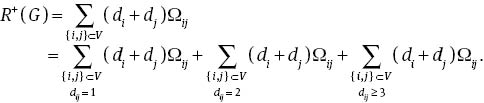
By the Foster formula [30], which states that the sum of resistance distances between pairs of adjacent vertices is equal to n – 1, we have

(14)∑{i,j} ⊂ Vdij = 1(di + dj)Ωij ≤ 2(n − 1)∑{i,j} ⊂ Vdij = 1Ωi,j = 2(n − 1)2. (14)

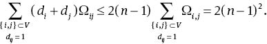
Then, by the fact that Ω_ij ≤ d_ij, it follows that

(15)∑{i,j} ⊂ Vdij = 2(di + dj)Ωij ≤ 2∑{i,j} ⊂ Vdij = 2(di + dj) ≤ 2(n − 1 + n − 1)∑{i,j} ⊂ Vdij = 21≤ 4(n − 1)[(n2) − (n − 1)]. (15)

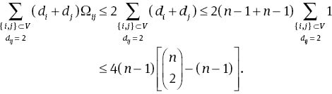
For i, j∈V such that d_ij ≥ 3, since i and j have no common neighbours, it follows that

dij ≤ n + 1 − (di + dj),

which gives

(di + dj)Ωij ≤ (di + dj)dij ≤ (di + dj)[n − 1 − (di + dj)] ≤ (n − 1)24.

Noting that pairs of vertices at distance 3 is less than or equal to

n(n − 1)2 − (n − 1) = (n − 2)(n − 1)2,

it follows that

(16)∑{i,j} ⊂ Vdij ≥ 3(di + dj)Ωij ≤ (n − 1)24∑{i,j} ⊂ Vdij ≥ 31 = (n − 1)24(n − 2)(n − 1)2 = (n − 2)(n − 1)38. (16)

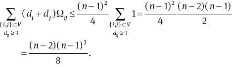
Substitution of (14)–(16) back into (13) yields the desired result.

Equality in (14) holds only when the end vertices of each edge of G are n – 1, which means G is n – 1 regular, in other words, G is a complete graph. On the other hand, equality in (15) holds also requires that G has n – 1 edges, which indicates G is a tree. Thus, equality in Theorem 9 holds only when G ≅ K₂, and it is easily verified that R⁺(K₂) does attain the upper bound.

References

[1] D. J. Klein and M. Randić, J. Math. Chem. 12, 81 (1993).10.1007/BF01164627Search in Google Scholar
[2] A. Ghosh, S. Boyd, and A. Saberi, SIAM Rev. 50, 37 (2008).10.1137/050645452Search in Google Scholar
[3] W. Ellens, F. M. Spieksma, P. Van Mieghem, A. Jamakovic, and R. E. Kooij, Linear Algebra Appl. 435, 2491 (2011).10.1016/j.laa.2011.02.024Search in Google Scholar
[4] H. Chen and F. Zhang, Discrete Appl. Math. 155, 654 (2007).10.1016/j.dam.2006.09.008Search in Google Scholar
[5] I. Gutman, L. Feng, and G. Yu, Trans. Comb. 1, 27 (2012).Search in Google Scholar
[6] M. Bianchi, A. Cornaro, J. L. Palacios, and A. Torriero, J. Math. Chem. 51, 569 (2013).10.1007/s10910-012-0103-xSearch in Google Scholar
[7] N. Chair, Ann. Phys. 341, 56 (2014).10.1016/j.aop.2013.11.012Search in Google Scholar
[8] K. C. Das, Z. Naturforsch. 68a, 531 (2013).Search in Google Scholar
[9] Q. Deng and H. Chen, Linear Algebra Appl. 439, 167 (2013).10.1016/j.laa.2013.03.009Search in Google Scholar
[10] Q. Deng and H. Chen, Linear Algebra Appl. 444, 89 (2014).10.1016/j.laa.2013.11.038Search in Google Scholar
[11] R. Li, MATCH-Commun. Math. Co. 70, 163 (2013).10.4028/www.scientific.net/AMR.827.163Search in Google Scholar
[12] J. Liu, J. Cao, X. Pan, and A. Elaiw, Discrete Dyn. Nat. Soc. 2013, 7 p. (2013), Article ID 543189.10.1155/2013/543189Search in Google Scholar
[13] J. Liu, X. Pan, Y. Wang, and J. Cao, Math. Probl. Eng. 2014, 9 p. (2014), Article ID 380874.Search in Google Scholar
[14] A. Nikseresht and Z. Sepasdar, Electron J. Comb. 21, P1.25 (2014).10.37236/3508Search in Google Scholar
[15] W. Wang, D. Yang, and Y. Luo, Discrete Appl. Math. 161, 3063 (2013).10.1016/j.dam.2013.06.010Search in Google Scholar
[16] Y. Yang, Discrete Appl. Math. 171, 153 (2014).10.1016/j.dam.2014.02.015Search in Google Scholar
[17] Y. Yang and D. J. Klein, Discrete Appl. Math. 175, 87 (2014).10.1016/j.dam.2014.05.014Search in Google Scholar
[18] Y. Yang and D. J. Klein, Discrete Appl. Math. 181, 260 (2015).10.1016/j.dam.2014.08.039Search in Google Scholar
[19] Z. Zhang, J. Stat. Mech. 2013, P10004 (2013).10.1088/1742-5468/2013/10/P10004Search in Google Scholar
[20] M. Bianchi, A. Cornaro, J. L. Palacios, and A. Torriero, Croat. Chem. Acta 86, 363 (2013).10.5562/cca2282Search in Google Scholar
[21] J. L. Palacios, MATCH-Commun. Math. Co. 70, 651 (2013).Search in Google Scholar
[22] A. Ben-Israel and T. N. E. Greville, Generalized Inverses: Theory and Applications, 2nd ed., Springer, New York 2003.Search in Google Scholar
[23] I. Gutman and B. Mohar, J. Chem. Inf. Comput. Sci. 36, 982 (1996).10.1021/ci960007tSearch in Google Scholar
[24] D. J. Klein, MATCH-Commun. Math. Co. 35, 7 (1997).10.1007/978-3-322-96937-8_6Search in Google Scholar
[25] D. Stevanović, MATCH-Commun. Math. Co. 60, 71 (2008).Search in Google Scholar
[26] A. Ilic, Linear Algebra Appl. 431, 2203 (2009).10.1016/j.laa.2009.07.022Search in Google Scholar
[27] H. Zhang and Y. Yang, Int. J. Quantum Chem. 107, 330 (2007).10.1002/qua.21068Search in Google Scholar
[28] Y. Yang and H. Zhang, J. Phys. A: Math. Theor. 41, 445203 (2008).10.1088/1751-8113/41/44/445203Search in Google Scholar
[29] H. Chen and F. Zhang, J. Math. Chem. 44, 405 (2008).10.1007/s10910-007-9317-8Search in Google Scholar
[30] R. M. Foster, The average impedance of an electrical network, in: Contributions to Applied Mechanics (Ed. J. W. Edwards), Edwards Brothers, Inc., Ann Arbor, MI 1949, pp. 333–340.Search in Google Scholar
©2015 by De Gruyter
Articles in the same Issue
- Frontmatter
- A Note on Exact Solutions for the Unsteady Free Convection Flow of a Jeffrey Fluid
- Equation of State, Nonlinear Elastic Response, and Anharmonic Properties of Diamond-Cubic Silicon and Germanium: First-Principles Investigation
- Quantum Electron-Exchange Effects on the Buneman Instability in Quantum Plasmas
- Diffraction of Pulsed Sound Signals by Elastic Bodies of Analytical and Non-analytical Forms, Put in Plane Waveguide
- Density Functional Theory Calculations of H/D Isotope Effects on Polymer Electrolyte Membrane Fuel Cell Operations
- Rogue Waves and New Multi-wave Solutions of the (2+1)-Dimensional Ito Equation
- Direct Similarity Reduction and New Exact Solutions for the Variable-Coefficient Kadomtsev–Petviashvili Equation
- Application of Nuclear Quadrupole Resonance Relaxometry to Study the Influence of the Environment on the Surface of the Crystallites of Powder