Statistical models and computational algorithms for discovering relationships in microbiome data
-
Mateen R. Shaikh


Abstract
Microbiomes, populations of microscopic organisms, have been found to be related to human health and it is expected further investigations will lead to novel perspectives of disease. The data used to analyze microbiomes is one of the newest types (the result of high-throughput technology) and the means to analyze these data is still rapidly evolving. One of the distributions that have been introduced into the microbiome literature, the Dirichlet-Multinomial, has received considerable attention. We extend this distribution’s use uncover compositional relationships between organisms at a taxonomic level. We apply our new method in two real microbiome data sets: one from human nasal passages and another from human stool samples.
1 Introduction
Human microbiomes are populations of microscopic organisms which live on or in a person. These populations have been found to relate to some diseases, with some illnesses associated with dramatic changes in the microbiome (Cho and Blaser, 2012). Modern microbiome data is produced from next-generation sequencing technology, which is itself a challenging, developing area of research. When a biological sample for microbiome analysis is collected from a person, it does not contain sequences just from a single organism’s genome, but the genomes of many microscopic organisms, making the analysis metagenomic. Analyzing the metagenomic signature of a microbiome is wrought with the challenges of traditional sequencing technology and compounded by the medley of information created by sequencing many organisms at once. With a commonly used method, genetic sequences are returned without any indication whether some sequences even came from the same organisms, let alone from the same species. These unlabelled sequences can be compared to known sequences to categorize the sequence at higher taxonomic levels, such as the family or genus. An issue arises in classifying the species, however, as classical (e.g. plant and animal) definitions of species are inappropriate for bacteria. In light of this problem with the species-level taxa, a substitute taxonomic level is introduced and used instead to operate at approximately the same level as species. This so-called Operational Taxonomic Unit (OTU) is defined by sequence similarity.
Processing microbiome data results in a long list of sequences for every sample processed. As mentioned, these sequences can be aggregated to create a table tallying how many of each OTU was found in each sample. This OTU table forms the basis of many analyses. One approach is to analyze the relative proportions of each OTU within the sample. A natural distribution to model proportions is the multinomial distribution, a generalization of the binomial distribution. Unfortunately, microbiome data exhibit dramatic overdispersion for such a simple distribution, making any results using just the multinomial questionable. One approach to handle this overdispersion is through a more flexible variant of the distribution, the Dirichlet-Multinomial (DM; Mosimann, 1962) distribution. Several uses and extensions to the DM have been introduced in the microbiome literature for a variety of useful applications. A hypothesis test to see if the data are indeed suitably modelled by a DM was previously outlined (La Rosa et al., 2012). The DM has been used in sparse variable selection (Chen et al., 2013), and been advocated as a realistic means of simulating microbiome data (Chen et al., 2012). The DM has also been used in clustering algorithms to find structure using finite mixture models (FMMs; Holmes et al., 2012). A clear advantage of using FMMs of DM is that it can be flexible for modelling compositions of OTUs in samples. Since this approach can be used to model compositions, we may be interested in extending the method further not only to analyze compositions but determine relationships between the OTUs based on those compositions. In particular, we can focus on OTUs that exist in approximately the same proportions in samples.
To discover these relationships, we take further advantage of the DM in a data-driven approach by inferring 1) compositions through the model’s existing parameters, and 2) equalities amongst the compositions by (relative) equalities amongst the model’s parameters. This shifts the focus of previous applications of the DM from individual bacteria to the relationships between bacteria by discovering compositional similarities. We briefly outline the concept of our proposed method with the following scenario. Consider a DM modelling abundances of various bacteria across various biological samples. We may find that some species occur in approximately the same proportions as other species, even though the actual abundances vary between samples. We may then reasonably consider whether these compositional similarities indicate some relationship between species. This approach would also then have the statistical desirable property of resulting in a model with fewer free parameters with approximately the same quality of fit.
As mentioned, OTUs which exist in the same proportions may indicate some type of relationship. For instance, organisms which consume a common food source, sufficiently abundant that competition is not incited, could grow or maintain the same relative abundances. This could occur with genomically distinct organisms that are functionally similar in the microbiome. A related possibility is that instead of a common food source supplying these organisms directly, they supply some (chain of) intermediary organisms, which in turn, create products that the genomically distinct organisms consume. As a reviewer pointed out, this could be evidence of some type of mutualism between organisms. In the analysis of the nasal data, we show that the constraints we find correspond to organisms known to compete opportunistically against each other in the airways and simultaneously fought by the host immune system. We found this to be consistent with our goal of devising a statistical approach that reflects real biological phenomena.
To address the problem of finding constraints, we employ an evolutionary algorithm (EA), a procedure that finds solutions to problems that are “optimal” in some sense by randomly finding slightly “more optimal” solutions. This process will consider a small collection of pairs of OTUs and consider if they exist in approximately equivalent proportions. The best candidates pairs are maintained and new pairs are considered until new pairs are no more optimal than existing pairs. To our knowledge, this will be the first application of the DM solving this type of problem in a microbiome context, and we believe the first introduction of evolutionary algorithms to the microbiome literature. We will use this method to infer relationships between different OTUs and compare the results with a previous analysis on that data. We will also apply this method to data at another taxonomic level, showing a limitation that occurs when OTUs have been agglomerated.
The remainder of the manuscript is outlined as follows. In Section 2 we will discuss the data motivating this new approach. In Section 3, we will discuss our methodology, beginning with the necessary background information in Section 3.1, and then method development in Section 3.2. We will then briefly apply the method to a toy example to illustrate how to make inferences before applying it to the real data sets in the following sections. We end the manuscript with a discussion of the advantages and limitations of using our method to make inferences from microbiome data in Section 5.
2 Motivating examples
2.1 Nasal data
The first dataset motivating our methodology is a result of a study from data collected in 2011–2012 from the upper airways of 74 infants, 10 children, and 33 adults, from nasal (69) and oral (49) passages, totalling 118 samples. We will consider data from the 69 nasal samples (18 adults, six children, and 45 infants) here.
Detailed information on processing is available from the original publication (Stearns et al., 2015). Briefly, the v3 region of the 16S rRNA was amplified and sequenced using the Illumina MiSeq instrument and aligned with PANDASeq. Sequences were clustered into OTUs using AbundantOTU+ employing a 97% similarity threshold. Taxonomies were assigned to the genus by the pipeline Quantitative Insights Into Microbial Ecology (QIIME) using the Ribomosmal Database Project against the Greengenes reference database. OTUs that were not classified with a confidence of at least 0.8 in QIIME were excluded. This original study sought to discover differences in the upper repository tracts of children compared to adults. The authors discovered increases in both diversity and load of microbiome from a period of high risk for respiratory disease (childhood) to the a matured microbiome. This analysis employed a variety of methods including discovering differential abundance, comparing diversity, and other class comparison approaches, which is not the goal of our work.
2.2 Twins data
The second motivating data set is well-known in the microbiome data, used to analyze stool samples of lean and obese twins and their mothers (Turnbaugh et al., 2008), grouped at the genera level (Holmes et al., 2012). The original analysis discovered compositions and phylogenic similarities varied with consanguinity.
3 Methodology
Before introducing the proposed method itself, we first discuss the necessary technical detail of the background material used to develop the method. It briefly outlines the development of the DM, applications of FMMs and terminology of EAs.
3.1 Background
3.1.1 The Dirichlet-Multinomial distribution
The multinomial distribution is suitable for representing counts from a population where the probability of selecting a category, such as an OTU, remains (approximately) the same, independent of other selections, and the total number of selections is fixed. The multinomial probability mass function of the multinomial is given in Eq. (1)).
Here, xj is the number of times OTU j is observed among p different types of OTUs, ϕj is the probability of observing OTU j, and Γ is the gamma function. Note that we will use the common notation
To account for overdispersion, proportions may be considered to be random variables rather than fixed values. In this case, the distribution to model proportions is often the conjugate prior of the multinomial, the Dirichlet distribution, shown in Eq. (2),
where αj > 0 is a parameter dictating the dispersion of the proportion ϕj, and so it itself is a parameter associated with OTU j. A compound distribution results by multiplying the two and integrating out the random proportions over the unit p − 1 simplex, resulting in the DM of Eq. (3).
3.1.2 Finite mixture models
A finite mixture model (FMM) is a method of representing G distinct subpopulations, each of which can possess its own probability density (or mass) function, fg, for g = 1, 2, …, G. The probability function of the entire population can then be expressed as
3.1.3 Evolutionary algorithms
An evolutionary algorithm (EA) is a means of finding optimal solutions to a problem that mimics natural selection whereby organisms (possible solutions) with better genes (properties) are favoured over successive generations (iterations). A didactic example of an EA is the string evolver. Imagine one person (evaluator) has a seven-digit phone number in mind and another person (guesser) is trying to guess it but only knows the phone number is seven digits. The guesser begins by giving a collection of 10 randomly-generated seven-digit numbers to the evaluator who ranks the numbers from most correct to least correct and tells the guesser the ranking of each phone number based on how correct it is. The guesser discards the five worst phone numbers, replacing them with a copy of each of the five best. The guesser then has two copies of each of the five phone numbers, so one random digit in one of the two copies is changed to a random number. Now the guesser has 10 numbers which could all be distinct. The process of the evaluator rating the phone numbers repeats with the five best phone numbers being kept, copied, etc.. Eventually, the same five phone numbers will be returned in several successive iterations. These five phone numbers will be potential solutions the guesser has to the phone number the evaluator has in mind. Despite being random, this process of guessing a phone number is far more efficient than having the guesser ask the evaluator to individually rate all ten million possible random phone numbers (the brute-force approach).
As mentioned, EAs are inspired by the process of propagation and selection based on fitness, found in nature. Although we do not provide a complete summary of these class of algorithms, we briefly outline EAs and highlight some of the terminology (Ashlock, 2006) which was also the source motiving our string evolver example above. The reader is referred to this book or expert overviews and further reference (Bäck, 1996; Bäck and Schwefel, 1996) on EAs.
There are several key components to an EA which we will define here (and parenthetically illustrate from the string evolver example). All of these terms are in reference to the EA, not the biological context. Although not common in EA literature, we will append the word “evolutionary” or “EA” in front of EA terms where necessary to distinguish them from their biological counterparts. An evolutionary gene is a trait that can differ between solutions (one digit of the phone-number). An evolutionary organism is one potential solution comprised of genes (a complete phone number). Variational operators are methods of constructing new phone numbers. The only variational operator we considered in the phone number-example was mutation: altering exactly one gene in an organism (altering one digit). Offspring are the organisms resulting from the application of variational operators (new phone numbers resulting from copying old ones and changing a digit). Fitness is some value assigned to an organism for the purpose of selection, pruning away organisms based on fitness. In our example, the evaluator performed the task of evaluating the fitness of individuals for the purpose of pruning away the lowest five scoring phone numbers.
In our microbiome context, we will propose an EA where compositional similarities, represented by constraints in the statistical model, are the EA organisms and a standard statistical model-selection criterion is our method of selection. This is akin to stepwise selection in multiple linear regression, but stepwise selection is a special case of our method. Rather than constraints, the goal of stepwise selection is to determine a subset of potential predictors in a model by successively adding a predictor at every iteration. In stepwise selection, the case is special because every possible mutation (adding/removing a potential predictor from the model) is considered at every iteration, and only the single best organism (potential model with predictors) survives selection (based on some criterion like Bayesian Information Criterion; BIC) to form a new generation. This reduces the random process to a deterministic one once the algorithm begins in stepwise regression. However, the more general undermentioned algorithm should be considered stochastic.
3.2 Methods development
Our goal is to determine relationships amongst OTUs by analyzing potential constraints of a DM, in particular, a FMM of a DM. We will use nearly the same model as the previous FMM of a DM in the microbiome research (Holmes et al., 2012) with one difference. The original paper imposed prior distributions, altering the distribution of the data from a pure DM to one that is compounded with an inverse gamma. This was done because the multinomial distribution is a limiting case of the DM, occurring when the parameters tend to infinity, which clearly induces convergence issues. Imposing a prior on the parameters succeeds in quelling estimates to remain finite but removed this special case of the DM. This can alter our impression of the data by suggesting there is more dispersion than may actually exist in the data. Instead, we impose a very large cutoff value for the parameters that, when exceeded, the model is considered to be a pure multinomial distribution. This is analogous to simply approximating a t distribution with a normal distribution when the degrees of freedom is large.
The concept of using constrained models, especially in FMMs, has been explored in the literature numerous times. A famous implementation is MCLUST (Banfield and Raftery, 1993), implemented in R ((Fraley and Raftery, 1999, 2002). In that application, constraints on model parameters are used to simultaneously make the model more parsimonious while the constraints themselves are directly interpretable in a basic-science point of view. We are inspired by this approach as the parameter constraints (values of different α constrained to be equal) has biological meaning as OTU abundances are approximately equal.
3.2.1 EA construction
We will represent constraints through partitions of parameters where each partition has only one degree of freedom. If two parameters exist in the same partition, then their value is necessarily forced to be equal to each other. In an unconstrained model, every parameter is in a partition by itself. Every partition can be represented by sets of equalities between every pair of parameters. Thus, the EA organism, a particular set of constraints on the DM, is faithfully represented as a collection of EA genes: where an EA gene is a pairwise constraint. A mutation in the EA will be imposing a new constraint to the EA organism and we avoid null mutations by ensuring we only allow mutations which can change the organism. Note that in some instances, some additional equalities will be imposed by transitivity. For instance if α1 = α2 already in one candidate model at one stage of the EA and the constraint α2 = α3 is imposed on the model, the constraint α1 = α3 must automatically be imposed. All three OTUs represented by α1, α2 and α3 will be considered to exist in approximately the same proportions in the microbiome.
When a constraint is imposed, rather than replace the value of one parameter another and completely lose the information originally held by one parameter, we will replace both by the average of the two. In general, when any partition is formed, each parameter in the partition will be replaced by the arithmetic mean of original values of the parameters in the partition. This is intuitive but has a useful property specific to the DM in complete-data log-likelihood shown in Eq. (4).
Here, αgj is the parameter corresponding to OTU j in group g where the proportion of group g comprised of OTU j is
Our goal in finding compositional similarities in the microbiome is reflected by sufficiently similar parameters in the model which we will constrain to be equal. We make two notes which aids the development of our algorithm. First, any final collection of constraints can be decomposed into a set of pairwise constraints. Second, there exists a sequence (not necessarily unique) of successive pairwise constraints that can be added incrementally to an unconstrained model to arrive at any constrained model. Therefore, we will focus only on pairwise constraints and represent the final set of constraints as sets of pairwise constraints. Model similarity is again like the case of the t distribution. Two t distributions with a large difference in degrees of freedom can be considered to be approximately the same distribution when the degrees of freedom parameter from each respective distribution is large. The same difference in degrees of freedom, however, may not be acceptable to consider approximate equality if one of the degrees of freedom is small. For instance, the difference between t distributions with 105 and 115 degrees of freedom is often negligible but the difference between t distributions with 5 and 15 degrees of freedom is far more considerable. By way of this analogy, it should then make sense to declare two distributions sufficiently similar when the reciprocal difference is sufficiently close to zero. This shall be our approach to compare different distributions that differ only by one of the α parameters.
Given a candidate set of constraints, the complete-data log-likelihood is re-evaluated and the effective number of parameters in light of the constraints re-counted to estimate the BIC (Schwartz, 1978). We use the BIC because it is well understood and enforces fewer free parameters, which we prefer, than than other well-known criteria like the AIC. It has also specifically been favoured in the context of FMMs (Leroux, 1992; Keribin, 2000) for many reasons including as a model selection criterion ((Fraley and Raftery, 1998, 2002).
4 Examples
Before analyzing our motivating data, we illustrate our method using a small simulated data set. The purpose of this is to show how to make inferences from this method. We specifically explain how to interpret results in various forms of a symmetric heatmap with this simple data before using it on our more complicated, real data in following sections.
4.1 Simulated data
We construct 3 groups of data simulated from the DM distribution. Data were simulated using the dirmult package in R, an implementation of the method examining overdispersion in allelic counts (Tvedebrink, 2010). Simulating from the DM has been justified as a reasonable representation of abundances in microbiome communities (Chen et al., 2012) and so we take this suggestion in constructing our example. Twelve of the thirteen OTUs are designed to comprise of one of three proportions: 2.9%, 5.7%, and 11.4% of the microbiome. One OTU is purposely designed to occur in approximately 5.9% of samples, slightly different from one collection of parameters to investigate the algorithm’s behaviour.
If we strictly use black and white (equality and inequality, respectively), we would visualize parameter similarities as in Figure 1A with the order of OTUs along rows matching the order along columns. We have designed the last variable to be similar to the second collection of parameters, so we may reasonably also consider Figure 1B to be a valid solution. We can extend the interpretation from only black & white figures to include shades, where light shades represent very different parameter values and dark shades representing very similar parameter values.
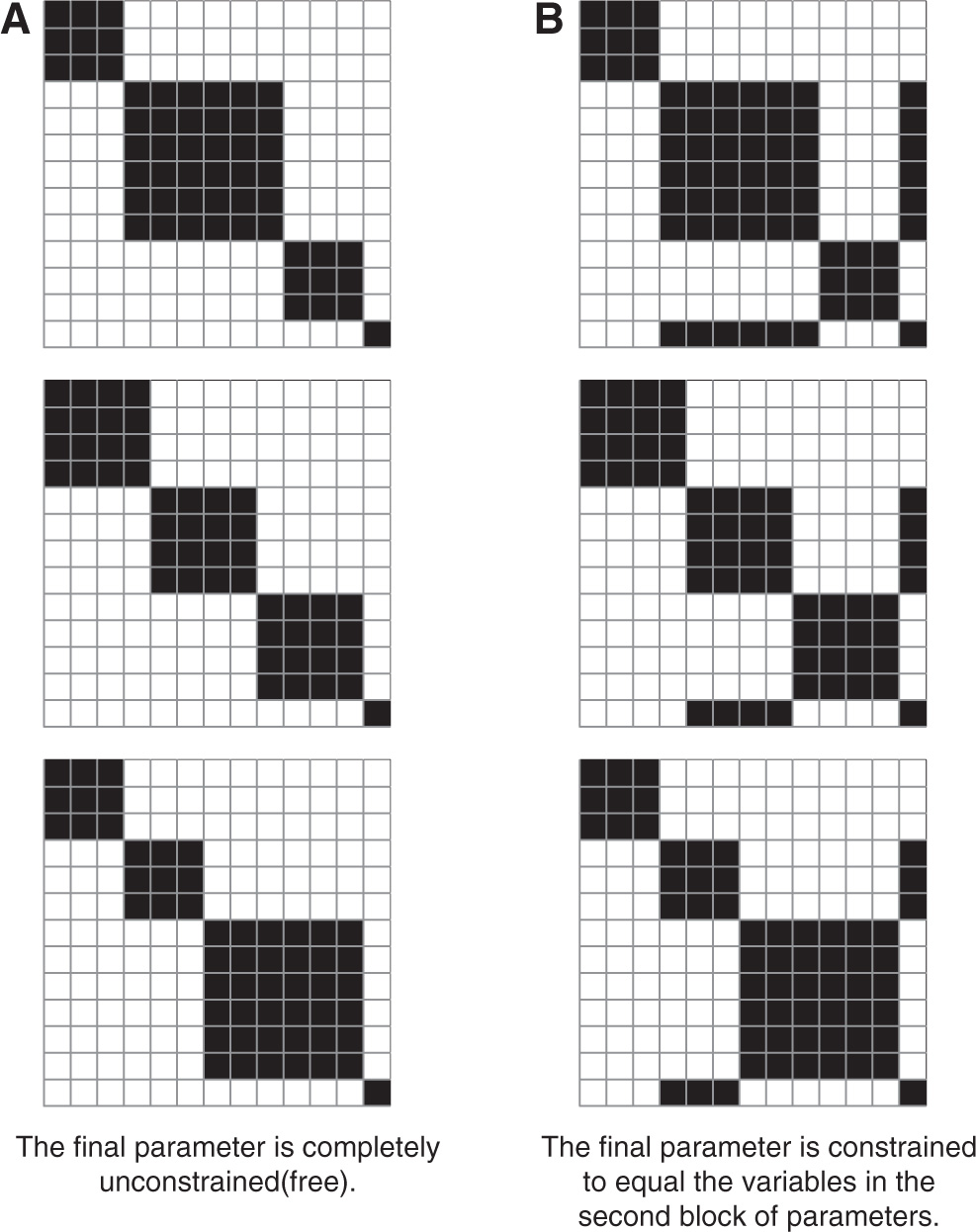
Heatmap representation of two potential solutions (sets of constraints) corresponding to the simulated data. The two solutions differ only by how the last variable is (un)constrained. (A) The final parameter is completely unconstrained (free). (B) The final parameter is constrained to equal the variables in the second block of parameters.
We run the EM algorithm ten times and choose the result with the best BIC. We illustrate the absolute reciprocal differences of the MLEs from the EM in Figure 2A. We can clearly see that although some semblances of group structure are apparent, it does not indicate which parameters should be strictly equal. We constructed an evolutionary algorithm and illustrate a sample organism from the evolved population in Figure 2B. The elements of this heatmap are dichotomous as it indicates whether the constraint between the two parameters was (or was not) imposed in this specific organism. Most, but not all, of the microbiome’s compositional similarity we are looking for are present in this one solution. Averaging over one evolved population, we see a result in Figure 2C that is more representative of the composition of our designed microbiome. Here, we see that based on the darkness of cells, more organisms from the evolved population imposed the constraint.
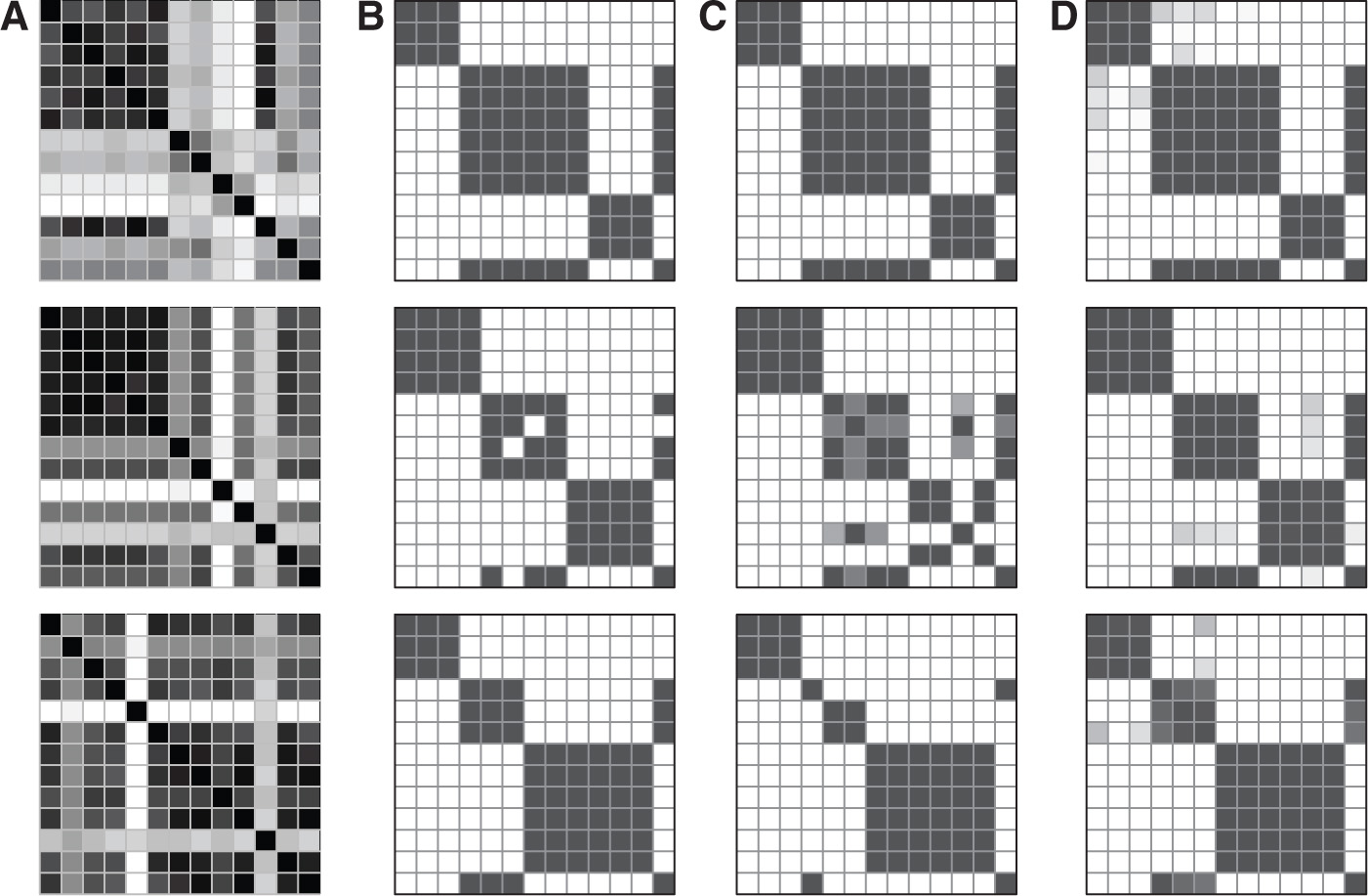
Progressively broader prospectives of results from the EA. (A) shows the estimated reciprocal differences of the true parameters. (B) shows an example of one organism of the converged population after running one EA. (C) shows the average organism from running one EA. (D) shows the average organism across twelve different runs of the EA.
As happens in biological evolution, a “founder effect” can considerably influence evolving populations. That is, randomly occurring common mutations which occur early during evolution can persist. To overcome this, we repeat the entire EA, allowing different mutations to evolve in each separate population. The result is shown in Figure 2D. We can see that a very good approximation to our original microbiome structure without having provided any input on what this structure should be. Therefore, we have found the compositional similarities in the microbiome that we had created by design without providing any semblence of that information to the algorithm.
With this example, we have illustrated that our method can faithfully determine how to reduce the number of free parameters of the DM by averaging over several restarted EAs. We will apply this procedure in the next example.
4.2 Nasal data
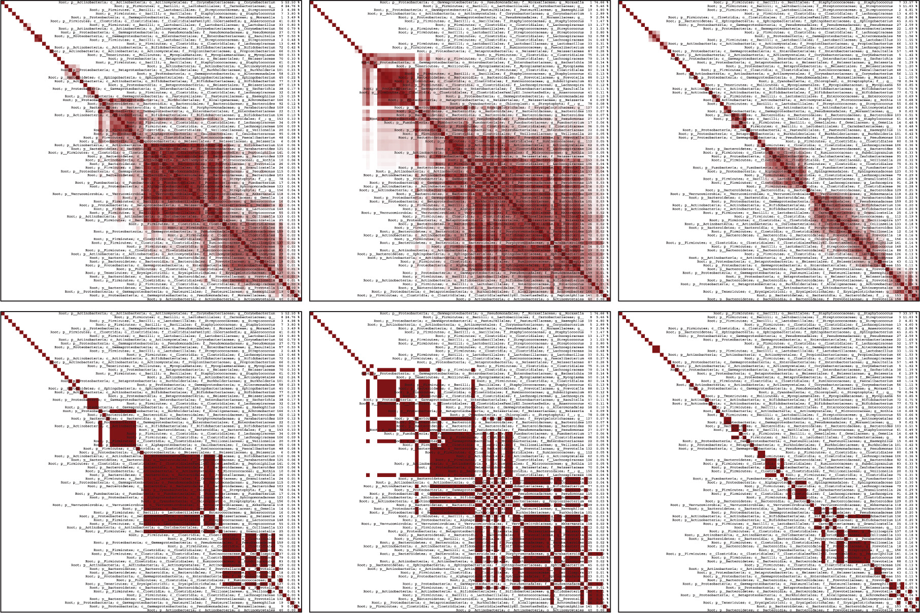
We run the EM algorithm and notice the value of the BIC increases as groups increase. Clearly the BIC alone as a selection technique is inadequate but because we plan to continue altering the model with the EA, we require some starting point. The three-component mixture model made groups of 16, 23, and 30 observations, which were very discernible: memberships of groups were very close to 1 or very close to 0, and never moderately in between. The largest jump in BIC occurs from two to three groups so we choose the three group model and to proceed to the EA. In this clustering, the first group was largely infants (12) but adults also contributed (4). In the second group, the group was largely infants (21) with very few children (2) and no adults. The third group was more heterogeneous with respect to age with infants (12) and children (4) and adults (14). As we will discuss below, this breakdown, particularly with the youngest group, is insightful in light of the discovered constraints. The resulting heatmaps are shown in Figure 3 and detailed information which lists the OTUs are shown in Figure 4 of Appendix A. OTUs are ordered by decreasing values of 𝜶 in heatmaps, which often (but interestingly, not always) correspond to where elements are grouped together.
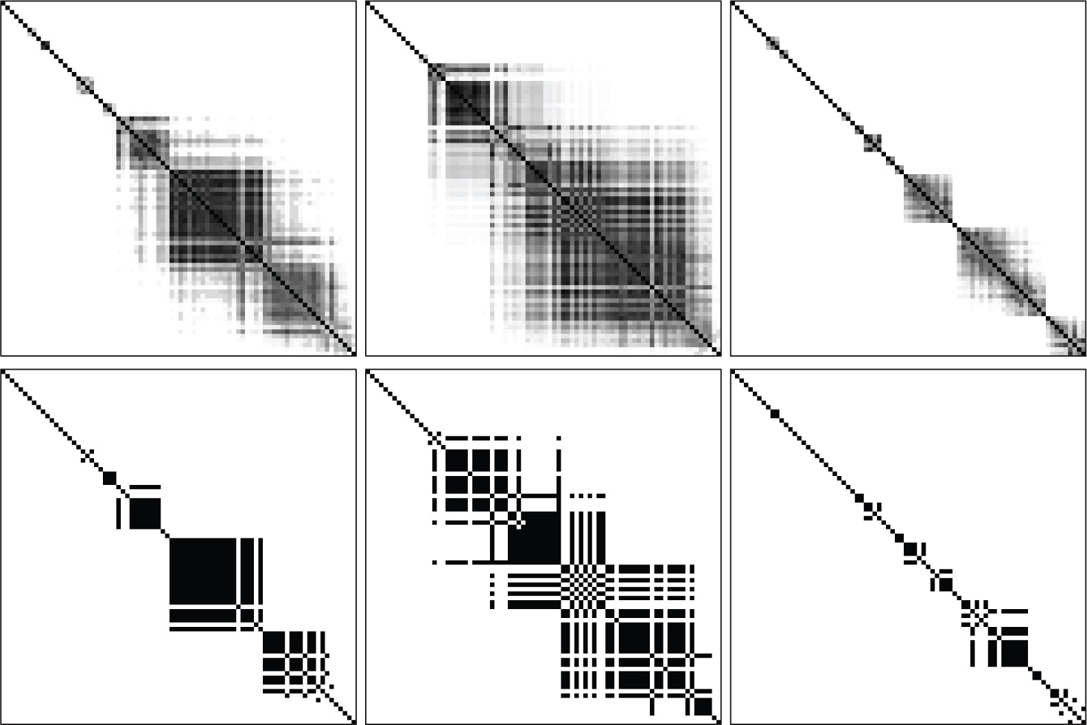
The top three heatmaps shows the averaged values and the bottom three of heatmaps shows the organism with the optimal BIC. A version with overlain phylogenic information labels is shown in Appendix A.
The top three heatmaps shows the averaged values and the bottom three of heatmaps shows the organism with the optimal BIC. Overlain is the corresponding phylogenic information.
The heatmap corresponding to the organism with the best BIC and the heatmap averaging over constraints are shown in Figure 3 and detailed information about the taxonomies are shown in Appendix A. Unlike the previous example, we see greater levels of uncertainty in the evolution as more moderate shades manifest. Nonetheless, we still observe several clear patterns. Not surprisingly, many of the parameters, which correspond to very few sequences found in the group per sample were grouped together, and therefore the freedom from the majority of parameters, which correspond to very few of the actual sequences is constrained, thereby increasing model fitness. This is not so surprising but what was more surprising was that not all of the low-abundant sequences were grouped into a single large group. The group that had high levels of Staphylococcus and Streptococcus, pathogenic genera (two left heatmaps), had the least constraints while the other groups not dominated by these genera.
Between the two heatmaps representing the organism with the best BIC and the average heatmap, some of the patterns are similar, but some are lost in one or the other heatmaps. For example, in the second group – the group which essentially contain no adults – there are two large sets of constraints which have the potential to overlap, and this is lost in the averaged heatmap as the two fuse together. Interestingly, this overlap corresponds to genera such as Prevotella and Fusobacterium. Prevotella is a genus known to be related to infections and disease (Schwarzberg et al., 2014). Although Fusobacterium has recently gained attention in the gut microbiome for recently being linked to colorectal carcinoma (Kostic et al., 2012), one species was already known to be linked to sepsis of the jugular vein, typically a result of oropharyngeal infection (Kuppalli et al., 2012) which makes sense as these samples are from nasal swabs. An OTU constrained to the same Prevotella was Haemophilus, which includes the species Haemophilus influenzae, an opportunistic pathogen that although common can cause disease in some conditions (Jurcisek and Bakaletz, 2007), including neonatal sepsis cases (Friesen and Cho, 1986; Kinney et al., 1993). These constraints occur specifically in a group dominated by Moraxella (which includes well-known pathogenic species (Verduin et al., 2002)), another OTU of Haemophilus, as well as genera known to include pathogenic organisms (Staphylococcus and Streptococcus). Many of these organisms are common but opportunistic, related to or even causing some illness, consistent with previous analysis that there seems to be a period at least among some children of a period of high risk for respiratory and related illness. This suggests that the constraints our methods find are biologically meaningful, as these opportunistic pathogens are often in direct competition with one another. It therefore seems that the growth during these opportunistic times are very related to each other.
4.3 Twins data
We used our novel approach to analyze the twins data set. Remarkably, we found that no constraints improved the model beyond a selection event and so the algorithm terminated quickly in all instances. The corresponding heatmaps were just diagonals, with constraints occurring randomly as artefacts of our founding populations and so we do not display them here. Given how much data is agglomerated at the genera level rather than with OTUs it is understandable that the model is unable to find entire genera that should exist at the same level as other genera. It may also be an indication that analyses at higher taxonomic levels lose enough information that the remaining information cannot highlight constraints. We consider this failure of constraint discovery as a useful property as there are real scenarios where the method fails to identify any constraints.
5 Discussion
In this manuscript, we have introduced the two concepts to the microbiome literature. First, we quantitatively explored compositional similarities in a novel manner by taking advantage of previously unused properties of a statistical model that has already found use in the microbiome literature. Second, we introduced the EA, which, to our knowledge, has never been used for microbiome analysis.
We used our method to show how OTUs corresponding to genera related to infection and disease appeared in very similar proportions and supports the message from the corresponding research regarding opportunistic organisms in respiratory microbiomes of the young. This approach fails, however, when information is agglomerated at the genera level, as shown in the twins data set. When data has been in a way that the likelihood function suffers too much to warrant suggesting whole genera that exist in the same proportions as each other. The approach we presented searched for constraints by allowing parameters of the DM to represent OTUs, and constraints to represent relationships between organisms in the biological sample.
Our approach has additional limitations as well. First, the method computationally expensive, though this can be somewhat alleviated as it is trivially parallelizable. Second, the microbiome is typically dominated by several OTUs, and all other OTUs occur in dramatically decreasing proportions. Rarer OTUs can have less weight in the BIC for model fit, though this is where most of the constraints occur. Therefore, another fitness function, namely something designed specifically for the microbiome and rare OTUs, could even more insightful. In light of the second example, if genera were desired to be constrained by compositional similarity, a criterion that penalizes free parameters even more can make the algorithm find constraints even among agglomerated data, as in the case of the twins data set example. Another limitation of the method we present regards the suitability of the DM model itself. Although it has been used in the microbiome literature, it itself has limitations that our algorithm would carry with it. In particular, the DM only permits negative correlations with data. Positive correlations do exist in microbiome data, and to an extent our algorithm indirectly finds them but a model for the microbiome that directly permits positive correlations would be more suitable. A natural candidate is the generalized DM (Connor and Mosimann, 1969) and although this distribution does have a far more flexible covariance structure, it has the severe limitation that variables must have a known, unique ordering used in analysis. Inferences made between different orderings can be incompatible, making it inappropriate in a microbiome setting. Therefore, an alternative distribution would more useful in microbiome analysis.
Funding source: Natural Sciences and Engineering Research Council of Canada
Award Identifier / Grant number: RGPIN 04360-2015
Funding statement: Natural Sciences and Engineering Research Council of Canada Discovery Grant: RGPIN 04360-2015, Canadian Institute of Health Research (Grant Number: 84392).
Acknowledgement
The authors would like to thank the anonymous referees for the valuable suggestions that improved this manuscript. The authors are also thankful to Drs. Michael Surette and Jennifer Stearns for the data and providing biological insights. This work was inspired by a collaboration which includes microbiome research, Canadian Institute for Health Research (RFA 201301FH6; 2013–2018) grant in Food & Health Population—Health Research.
Appendix A Detailed phylogenic information for nasal data
The detailed phylogenic information for the results from Section 4.2 is illustrated in Figure 3 is shown here in Figure 4. This is best viewed electronically due to the small font size.
References
Arumugam, M., J. Raes, E. Pelletier, D. Le Paslier, T. Yamada, D. R. Mende, G. R. Fernandes, J. Tap, T. Bruls, J.-M. Batto, M. Bertalan, N. Borruel, F. Casellas, L. Fernandez, L. Gautier, T. Hansen, M. Hattori, T. Hayashi, M. Kleerebezem, K. Kurokawa, M. Leclerc, F. Levenez, C. Manichanh, H. B. Nielsen, T. Nielsen, N. Pons, J. Poulain, J. Qin, T. Sicheritz-Ponten, S. Tims, D. Torrents, E. Ugarte, E. G. Zoetendal, J. Wang, F. Guarner, O. Pedersen, W. M. de Vos, S. Brunak, J. Doré, M. Consortium, J. Weissenbach, S. Dusko Ehrlich and P. Bork (2011): “Enterotypes of the human gut microbiome,” Nature, 473, 174–180.10.1038/nature09944Search in Google Scholar PubMed PubMed Central
Ashlock, D. (2006): Evolutionary computation for modeling and optimization, Springer.Search in Google Scholar
Bäck, T. (1996): Evolutionary algorithms in theory and practice: evolution strategies, evolutionary programming, genetic algorithms, Oxford University Press.10.1093/oso/9780195099713.001.0001Search in Google Scholar
Bäck, T. and H.-P. Schwefel (1996): “Evolutionary computation: An overview,” in Evolutionary Computation, 1996., Proceedings of IEEE International Conference on, IEEE, 20–29.10.1109/ICEC.1996.542329Search in Google Scholar
Banfield, J. D. and A. E. Raftery (1993): “Model-based Gaussian and non-Gaussian clustering,” Biometrics, 49, 803–821.10.2307/2532201Search in Google Scholar
Chen, J., K. Bittinger, E. S. Charlson, C. Hoffmann, J. Lewis, G. D. Wu, R. G. Collman, F. D. Bushman and H. Li (2012): “Associating microbiome composition with environmental covariates using generalized unifrac distances,” Bioinformatics, 28, 2106–2113.10.1093/bioinformatics/bts342Search in Google Scholar PubMed PubMed Central
Chen, J. and H. Li (2013): “Variable selection for sparse Dirichlet-multinomial regression with an application to microbiome data analysis,” Ann. Appl. Stat., 7, 418–442.10.1214/12-AOAS592Search in Google Scholar PubMed PubMed Central
Cho, I. and M. J. Blaser (2012): “The human microbiome: at the interface of health and disease,” Nature Rev. Genet., 13, 260–270.10.1038/nrg3182Search in Google Scholar PubMed PubMed Central
Connor, R. J. and J. E. Mosimann (1969): “Concepts of independence for proportions with a generalization of the dirichlet distribution,” J. Am. Stat. Assoc., 64, 194–206.10.1080/01621459.1969.10500963Search in Google Scholar
Dempster, A. P., N. M. Laird and D. B. Rubin (1977): “Maximum likelihood from incomplete data via the EM algorithm,” J. R. Stat. Soc. Series B, 39, 1–38.10.1111/j.2517-6161.1977.tb01600.xSearch in Google Scholar
Fraley, C. and A. E. Raftery (1998): “How many clusters? Which clustering methods? Answers via model-based cluster analysis,” Comput. J., 41, 578–588.10.1093/comjnl/41.8.578Search in Google Scholar
Fraley, C. and A. E. Raftery (1999): “MCLUST: Software for model-based cluster analysis,” J. Classif., 16, 297–306.10.1007/s003579900058Search in Google Scholar
Fraley, C. and A. E. Raftery (2002): “Model-based clustering, discriminant analysis, and density estimation,” J. Am. Stat. Assoc., 97, 611–631.10.1198/016214502760047131Search in Google Scholar
Friesen, C. A. and C. T. Cho (1986): “Characteristic features of neonatal sepsis due to haemophilus influenzae,” Rev. Infect. Dis., 8, 777–780.10.1093/clinids/8.5.777Search in Google Scholar
Holmes, I., K. Harris and C. Quince (2012): “Dirichlet multinomial mixtures: generative models for microbial metagenomics,” PLoS One, 7, e30126.10.1371/journal.pone.0030126Search in Google Scholar
Jurcisek, J. A. and L. O. Bakaletz (2007): “Biofilms formed by nontypeable haemophilus influenzae in vivo contain both double-stranded dna and type iv pilin protein,” J. Bacteriol., 189, 3868–3875.10.1128/JB.01935-06Search in Google Scholar
Keribin, C. (2000): “Consistent estimation of the order of mixture models,” Sankhyā. Indian J. Statist. Series A, 62, 49–66.Search in Google Scholar
Kinney, J. S., K. Johnson, C. Papasian, R. T. Hall, C. G. Kurth and M. A. Jackson (1993): “Early onset haemophilus influenzae sepsis in the newborn infant.” Pediatr. Infect. Dis. J., 12, 739–742.10.1097/00006454-199309000-00007Search in Google Scholar
Kostic, A. D., D. Gevers, C. S. Pedamallu, M. Michaud, F. Duke, A. M. Earl, A. I. Ojesina, J. Jung, A. J. Bass, J. Tabernero, J. Baselga, C. Liu, R. A. Shivdasani, S. Ogino, B. W. Birren, C. Huttenhower, W. S. Garrett and M. Meyerson (2012): “Genomic analysis identifies association of fusobacterium with colorectal carcinoma,” Genome Res., 22, 292–298.10.1101/gr.126573.111Search in Google Scholar
Kuppalli, K., D. Livorsi, N. J. Talati and M. Osborn (2012): “Lemierre’s syndrome due to fusobacterium necrophorum,” Lancet Infect. Dis., 12, 808–815.10.1016/S1473-3099(12)70089-0Search in Google Scholar
La Rosa, P. S., J. P. Brooks, E. Deych, E. L. Boone, D. J. Edwards, Q. Wang, E. Sodergren, G. Weinstock and W. D. Shannon (2012): “Hypothesis testing and power calculations for taxonomic-based human microbiome data,” PLoS One, 7, e52078.10.1371/journal.pone.0052078Search in Google Scholar PubMed PubMed Central
Leroux, B. G. (1992): “Consistent estimation of a mixing distribution,” Ann. Stat., 20, 1350–1360.10.1214/aos/1176348772Search in Google Scholar
McLachlan, G. J. and D. Peel (2000): Finite mixture models, New York: John Wiley & Sons.10.1002/0471721182Search in Google Scholar
Mosimann, J. E. (1962): “On the compound multinomial distribution, the multivariate β-distribution, and correlations among proportions,” Biometrika, 49, 65–82.10.1093/biomet/49.1-2.65Search in Google Scholar
Schwartz, G. (1978): “Estimating the dimension of a model,” Ann. Stat., 6, 31–38.10.1214/aos/1176344136Search in Google Scholar
Schwarzberg, K., R. Le, B. Bharti, S. Lindsay, G. Casaburi, F. Salvatore, M. H. Saber, F. Alonaizan, J. Slots, R. A. Gottlieb, J. G. Caporaso and S. T. Kelley (2014): “The personal human oral microbiome obscures the effects of treatment on periodontal disease,” PLoS One, 9, e86708.10.1371/journal.pone.0086708Search in Google Scholar PubMed PubMed Central
Stearns, J. C., C. J. Davidson, S. McKeon, F. J. Whelan, M. E. Fontes, A. B. Schryvers, D. M. Bowdish, J. D. Kellner and M. G. Surette (2015): “Culture and molecular-based profiles show shifts in bacterial communities of the upper respiratory tract that occur with age,” ISME J., 9, 1246–1259.10.1038/ismej.2014.250Search in Google Scholar PubMed PubMed Central
Turnbaugh, P. J., M. Hamady, T. Yatsunenko, B. L. Cantarel, A. Duncan, R. E. Ley, M. L. Sogin, W. J. Jones, B. A. Roe, J. P. Affourtit, M. Egholm, M. Egholm, B. Henrissat, A. C. Heath, R. Knight and J. I. Gordon (2008): “A core gut microbiome in obese and lean twins,” Nature, 457, 480–484.10.1038/nature07540Search in Google Scholar PubMed PubMed Central
Tvedebrink, T. (2010): “Overdispersion in allelic counts and theta-correction in forensic genetics,” Theor. Popul. Biol., 78, 200–210.10.1016/j.tpb.2010.07.002Search in Google Scholar PubMed
Verduin, C. M., C. Hol, A. Fleer, H. van Dijk and A. van Belkum (2002): “Moraxella catarrhalis: from emerging to established pathogen,” Clin. Microbiol. Rev., 15, 125–144.10.1128/CMR.15.1.125-144.2002Search in Google Scholar PubMed PubMed Central
©2017 Walter de Gruyter GmbH, Berlin/Boston
Articles in the same Issue
- Frontmatter
- Research Articles
- Statistical models and computational algorithms for discovering relationships in microbiome data
- Binary Markov Random Fields and interpretable mass spectra discrimination
- Comparison and visualisation of agreement for paired lists of rankings
- Bivariate Poisson models with varying offsets: an application to the paired mitochondrial DNA dataset
- Generalized partial linear varying multi-index coefficient model for gene-environment interactions
- Software and Application Note
- Polyunphased: an extension to polytomous outcomes of the Unphased package for family-based genetic association analysis