Comparison and visualisation of agreement for paired lists of rankings
-
Margaret R. Donald
 and
Susan R. Wilson
and
Susan R. Wilson

Abstract:
Output from analysis of a high-throughput ‘omics’ experiment very often is a ranked list. One commonly encountered example is a ranked list of differentially expressed genes from a gene expression experiment, with a length of many hundreds of genes. There are numerous situations where interest is in the comparison of outputs following, say, two (or more) different experiments, or of different approaches to the analysis that produce different ranked lists. Rather than considering exact agreement between the rankings, following others, we consider two ranked lists to be in agreement if the rankings differ by some fixed distance. Generally only a relatively small subset of the k top-ranked items will be in agreement. So the aim is to find the point k at which the probability of agreement in rankings changes from being greater than 0.5 to being less than 0.5. We use penalized splines and a Bayesian logit model, to give a nonparametric smooth to the sequence of agreements, as well as pointwise credible intervals for the probability of agreement. Our approach produces a point estimate and a credible interval for k. R code is provided. The method is applied to rankings of genes from breast cancer microarray experiments.
Acknowledgement
This study was supported by the National Health and Medical Research Council (NHMRC grant # 525453). Comments by a reviewer substantially improved the paper.
Conflict of interest statement: None declared.
Appendix A: Technical details
A.1 Finding k, and its 95% credible intervals
The smoothing function, pj = 1/(1 + exp(−μj)) where μj = Xβ + Zu and j = 1, …, N, forms the basis for finding k and its credible interval. Let the sample of pj at iteration t (of T samples) in the MCMC process be pjt. We monitor pjt, thus giving T posterior MCMC samples of pjt from which we estimate pj and its 95% credible intervals. The posterior credible interval for k is found by post processing the posterior distributions pjt, to find kt at each (post burn-in) iteration, t. Thus, to find k, for each iteration, we perform the following calculation:
If p1t ≤ 0.5, then kt = 0; else
find the first jt, for which
if there is no jt, for which
That is, kt is the last value of j before pjt becomes less than 0.5. See the post processing R-code below.
A fundamental output of the method is a figure showing the pointwise estimates of pj (the median of pj) and their 95% credible intervals. We graph the pointwise 95% credible intervals as a shaded area, and join the medians with a dashed line. A horizontal solid line shows the 95% credible interval for k, which does not necessarily correspond to the shaded interval at probability = 0.5, but is calculated from the posterior distribution of k.
A.2 Calculation of effective degrees of freedom and the spline penalty
When fitting splines, one needs to know whether sufficient knots have been fitted. Does the model adequately fit the data? The sensitivity of the model to the choice of the number of degrees of freedom can be checked by fitting models with various degrees of freedom. Marley and Wand (2010), in a different context, suggest that 25 degrees of freedom should be adequate. Here with sequences of length often greater than 1000, more knots may well be needed. (Ruppert, 2002; Wang et al., 2011) suggest that 40 knots may be adequate, however large N may be.)
We find the estimated degrees of freedom (edf) for the spline model fit as follows. Adapting Marley and Wand (2010); Wand (2014), the design matrix for penalized spline fit is W = [X Z], κ is the number of internal knots, and N is the length of the sequence. Let
Then the effective degrees of freedom, edf, derived from Ruppert et al. (2003), Marley and Wand (2010) is given by:
The edf,
When the fitted degrees of freedom well exceeds the estimated degrees of freedom, it is clear that the smoothing has not been constrained by the choice of the number of fitted degrees of freedom.
BUGS code for penalized spline logit model
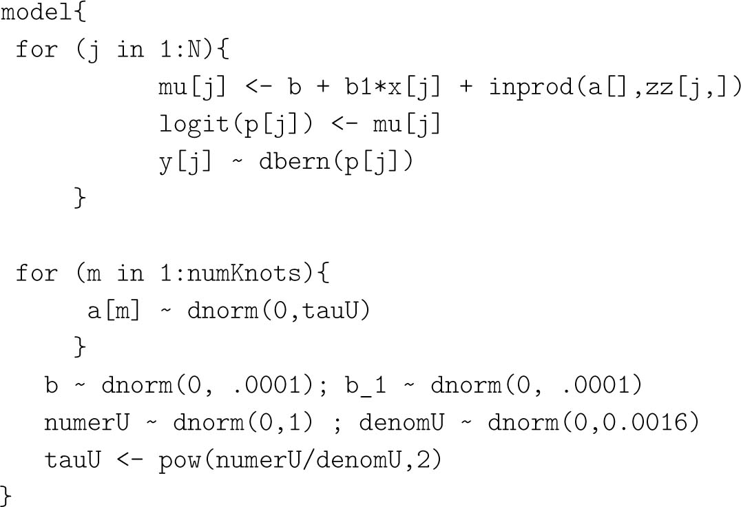
The code is valid in WinBUGS, OpenBUGS or JAGS.
The model uses a Half-Cauchy prior for the variance of the coefficients for the penalized spline terms. Marley and Wand (2010) recommend these and in our experience, they work well, allowing the model to initialize and adapt with no problems, while being uninformative. Code to generate the O’Sullivan splines over the number of knots for the predictor x is available from Wand and Ormerod (2008). When there are κ internal knots the fitted number of degrees of freedom (df) is κ + 4.
The last two lines of code show the technique for producing a Half-Cauchy(A) prior for
The code is valid for OpenBUGS, WinBUGS, and JAGS.
A.3 R code for calculating k and its 95% credible interval
Let
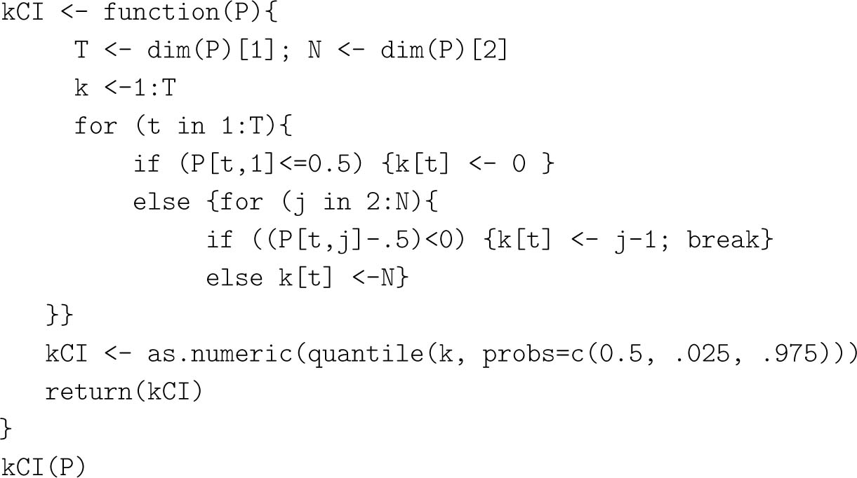
Thus, we search through the iterations to find the first j for which Ptj is less then 0.5. The tth sample of k, kt, is given by the value j − 1. At this point we exit the inner loop and return to the outer loop to find the next sample of k.
Note that if Pt1 is less than or equal to 0.5 in iteration, t, then kt is taken to be 0. If PtN is greater than 0.5 at iteration t, when j = N, then kt is taken to be N.
A.4 Further implementation details
For any given comparison, the agreement sequence is calculated using the TopKLists (Schimek et al., 2015b) function prepare.idata, which takes the two ranked lists and the desired distance, δ, to give the agreement sequence. The TopKLists function is used to ensure that agreement sequences are identical thereby allowing comparison with the estimated k from TopKLists. The spline bases are calculated via R code (ZOSull.R) supplied in Marley and Wand (2010). A function, wrapper(), outputs k and its credible intervals, together with pj and its summary statistics, and various graphs to a nominated subdirectory. Input parameters are the set of ranked data (in the form used by TopKLists), the two columns to be compared, and the distance (δ) desired for defining agreement of ranks.
The models were fit using R2jags (Su and Yajima, 2015) which uses JAGS (Plummer, 2011). Models were also fit using BRugs (Thomas et al., 2006). However, the R2jags framework was found to be both considerably faster, and more flexible in that it allowed easy random initializations of several chains.
In JAGS, burn-in was 10,000, and the number of posterior MCMC iterations for estimation was 15,000. Autocorrelation graphs, mixing graphs and distribution plots for various parameters were plotted and found to be satisfactory. The models showed good mixing and autocorrelation properties.
Appendix B: Supplementary files
R code Vignette: RankAgreeVignetteV10.pdf: A vignette outlining the code needed to run the wrapper function and necessary ancillary code.
VignetteScriptV4.R: R code for the vignette.
functions_kpV10.R: The code for the wrapper function and other necessary functions. The code for ZOSull.R which generates the O’Sullivan spline bases is found at http://www.jstatsoft.org/article/view/v037i05 (Marley and Wand, 2010).
MCMCSupportingFunctions.R: Supporting functions which take the MCMC objects from jags and graph the estimated probability function, together with some diagnostic graphs and csv files summarising the probability functions.
References
Antosh, M., D. Fox, L. N. Cooper and N. Neretti (2013): “CORaL: comparison of ranked lists for analysis of gene expression data,” J. Comput. Biol., 20, 433–443. http://dx.doi.org/10.1089/cmb.2013.0017.10.1089/cmb.2013.0017Search in Google Scholar PubMed PubMed Central
Crainiceanu, C. M., D. Ruppert and M. P. Wand (2005): “Bayesian analysis for penalized spline regression using WinBUGS,” J. Stat. Softw., 14, 1–24. http://www.jstatsoft.org/v14/i14/paper.10.18637/jss.v014.i14Search in Google Scholar
Desmedt, C., F. Piette, S. Loi, Y. Wang, F. Lallemand, B. Haibe-Kains, G. Viale, M. Delorenzi, Y. Zhang, M. S. d’Assignies, J. Bergh, R. Lidereau, P. Ellis, A. L. Harris, J. G. Klijn, J. A. Foekens, F. Cardoso, M. J. Piccart, M. Buyse and C. Sotiriou (2007): “Strong time dependence of the 76-gene prognostic signature for node-negative breast cancer patients in the transbig multicenter independent validation series,” Clin. Cancer Res., 13, 3207–3214.10.1158/1078-0432.CCR-06-2765Search in Google Scholar PubMed
Dobson, A. J. and A. G. Barnett (2008): An introduction to generalized linear models, Chapman & Hall/CRC Texts in statistical science series, vol. 77, Boca Raton: CRC Press, 3rd edition.Search in Google Scholar
Eden, E., D. Lipson, S. Yogev and Z. Yakhini (2007): “Discovering motifs in ranked lists of DNA sequences,” PLoS Comput. Biol., 3, e39, http://dx.plos.org/10.1371.10.1371/journal.pcbi.0030039Search in Google Scholar PubMed PubMed Central
Eden, E., R. Navon, I. Steinfeld, D. Lipson and Z. Yakhini (2009): “GOrilla: a tool for discovery and visualization of enriched GO terms in ranked gene lists,” BMC Bioinformatics, 10, 48, http://www.biomedcentral.com/1471-2105/10/48.10.1186/1471-2105-10-48Search in Google Scholar PubMed PubMed Central
Hall, P. and M. G. Schimek (2012): “Moderate-deviation-based inference for random degeneration in paired rank lists,” J. Am. Stat. Assoc., 107, 661–672.10.1080/01621459.2012.682539Search in Google Scholar
Hastie, T. and R. Tibshirani (1990): Generalized additive models, Monographs on statistics and applied probability, London, New York: Chapman and Hall, 1st edition.Search in Google Scholar
Lottaz, C., X. Yang, S. Scheid and R. Spang (2006): “Orderedlist - a Bioconductor package for detecting similarity in ordered gene lists,” Bioinformatics, 22, 2315–2316, http://bioinformatics.oxfordjournals.org/content/22/18/2315.abstract.10.1093/bioinformatics/btl385Search in Google Scholar PubMed
Lunn, D., C. Jackson, N. Best, A. Thomas and D. Spiegelhalter (2013): The BUGS book: a practical introduction to Bayesian analysis, Texts in statistical science, Boca Raton, FL: CRC Press.10.1201/b13613Search in Google Scholar
Mallows, C. L. (1957): “Non-null ranking models. I,” Biometrika, 44, 114–130, http://www.jstor.org/stable/2333244.10.1093/biomet/44.1-2.114Search in Google Scholar
MAQC Consortium (2006): “The microarray quality control (MAQC): project shows inter- and intraplatform reproducibility of gene expression measurements,” Nat. Biotechnol., 24, 1151 – 1161, http://www.nature.com/nbt/journal/v24/n9/full/nbt1239.html.Search in Google Scholar
Marley, J. K. and M. P. Wand (2010): “Non-standard semiparametric regression via BRugs,” J. Stat. Softw., 37, 1–30, http://www.jstatsoft.org/article/view/v037i05, http://www.jstatsoft.org/article/view/v037i05.10.18637/jss.v037.i05Search in Google Scholar
McCullagh, P. and J. A. Nelder (1989): Generalized linear models, Monographs on statistics and applied probability, vol. 37, London, New York: Chapman and Hall, 2nd edition.10.1007/978-1-4899-3242-6Search in Google Scholar
Mood, A. M. (1940): “The distribution theory of runs,” Ann. Math. Stat., 11, 367–392, http://www.jstor.org/stable/2235718.10.1214/aoms/1177731825Search in Google Scholar
O’Sullivan, F. (1986): “A statistical perspective on ill-posed inverse problems,” Stat. Sci., 1, 502–527, http://projecteuclid.org/euclid.ss/1177013525.10.1214/ss/1177013525Search in Google Scholar
Pihur, V., S. Datta and S. Datta (2014): RankAggreg: weighted rank aggregation, http://CRAN.R-project.org/package=RankAggreg, r package version 0.5.Search in Google Scholar
Pinheiro, J., D. Bates, S. DebRoy, D. Sarkar and R Core Team (2016): nlme: linear and nonlinear mixed effects models, http://CRAN.R-project.org/package=nlme, r package version 3.1-128.Search in Google Scholar
Plaisier, S. B., R. Taschereau, J. A. Wong and T. G. Graeber (2010): “Rank-rank hypergeometric overlap: identification of statistically significant overlap between gene-expression signatures,” Nucleic Acids Res., 38, e169, http://nar.oxfordjournals.org/content/38/17/e169.abstract.10.1093/nar/gkq636Search in Google Scholar PubMed PubMed Central
Plummer, M. (2011): JAGS Version 3.1. 0 user manual, http://gentoo.mirrors.lug.ro/freebsd/distfiles/mcmc-jags/jags_user_manual.pdf.Search in Google Scholar
Risso, D., J. Ngai, T. P. Speed and S. Dudoit (2014): “Normalization of RNA-seq data using factor analysis of control genes or samples,” Nat. Biotechnol., 32, 896–902.10.1038/nbt.2931Search in Google Scholar PubMed PubMed Central
Rubin, H. and J. Sethuraman (1965): “Probabilities of moderate deviations,” Sankhya Indian J. Stat. Ser. A (1961–2002), 27, 325–346.Search in Google Scholar
Ruppert, D. (2002): “Selecting the number of knots for penalized splines,” J. Comput. Graph. Stat., 11, 735–757.10.1198/106186002853Search in Google Scholar
Ruppert, D., M. P. Wand and R. J. Carroll (2003): Semiparametric regression, Cambridge series in statistical and probabilistic mathematics, Cambridge, UK: Cambridge University Press.10.1017/CBO9780511755453Search in Google Scholar
Schimek, M. G., E. Budinska, J. Ding, K. G. Kugler, V. Svendova and S. Lin (2015a): “TopKLists: analyzing multiple ranked lists,” https://cran.r-project.org/web/packages/TopKLists/vignettes/TopKLists.pdf.Search in Google Scholar
Schimek, M. G., E. Budinska, K. G. Kugler, V. Svendova, J. Ding and S. Lin (2014): “TopKLists show case for integrating miRNA measurements,” http://topklists.r-forge.r-project.org/showcase_miRNA/topklists-miRNA.html, accessed: August 25, 2016.Search in Google Scholar
Schimek, M. G., E. Budinska, K. G. Kugler, V. Svendova, J. Ding and S. Lin (2015b): “TopKLists: a comprehensive R package for statistical inference, stochastic aggregation, and visualization of multiple omics ranked lists,” Stat. Appl. Genet. Mol. Biol., 14, 311–316, https://www.degruyter.com/view/j/sagmb.2015.14.issue-3/sagmb-2014-0093/sagmb-2014-0093.xml.10.1515/sagmb-2014-0093Search in Google Scholar PubMed
Shannon, P., A. Markiel, O. Ozier, N. S. Baliga, J. T. Wang, D. Ramage, N. Amin, B. Schwikowski and T. Ideker (2003) “Cytoscape: a software environment for integrated models of biomolecular interaction networks,” Genome Res., 13, 2498–2504.10.1101/gr.1239303Search in Google Scholar PubMed PubMed Central
Stevens, W. L. (1939): “Distribution of groups in a sequence of alternatives,” Ann. Eugen., 9, 10–17, http://dx.doi.org/10.1111/j.1469-1809.1939.tb02193.x.10.1111/j.1469-1809.1939.tb02193.xSearch in Google Scholar
Su, Y.-S. and M. Yajima (2015): R2jags: using R to Run ‘JAGS’, http://CRAN.R-project.org/package=R2jags, R package version 0.5-6.Search in Google Scholar
Tabchy, A., V. Valero, T. Vidaurre, A. Lluch, H. Gomez, M. Martin, Y. Qi, L. J. Barajas-Figueroa, E. Souchon and C. Coutant (2010): “Evaluation of a 30-gene paclitaxel, fluorouracil, doxorubicin, and cyclophosphamide chemotherapy response predictor in a multicenter randomized trial in breast cancer,” Clin. Cancer Res., 16, 5351–5361.10.1158/1078-0432.CCR-10-1265Search in Google Scholar PubMed PubMed Central
Thomas, A., B. O’Hara, U. Ligges and S. Sturtz (2006): “Making BUGS open,” R News, 6, 12–17, http://cran.r-project.org/doc/Rnews/.Search in Google Scholar
Wand, M. P. (2009): “Semiparametric and graphical models,” Aust. N. Z. J. Stat., 51, 9–41.10.1111/j.1467-842X.2009.00538.xSearch in Google Scholar
Wand, M. P. (2014): Semiparametric regression (short course, UTS, Sydney), http://matt-wand.utsacademics.info/sprSC.html, July 11, 2014.Search in Google Scholar
Wand, M. P. and J. T. Ormerod (2008): “On semiparametric regression with O’Sullivan penalized splines,” Aust. N. Z. J. Stat., 50, 179–198.10.1111/j.1467-842X.2008.00507.xSearch in Google Scholar
Wang, X., J. Shen and D. Ruppert (2011): “On the asymptotics of penalized spline smoothing,” Electron. J. Stat., 5, 1–17.10.1214/10-EJS593Search in Google Scholar
Supplemental Material:
The online version of this article (DOI: 10.1515/sagmb-2016-0036) offers supplementary material, available to authorized users.
©2017 Walter de Gruyter GmbH, Berlin/Boston
Articles in the same Issue
- Frontmatter
- Research Articles
- Statistical models and computational algorithms for discovering relationships in microbiome data
- Binary Markov Random Fields and interpretable mass spectra discrimination
- Comparison and visualisation of agreement for paired lists of rankings
- Bivariate Poisson models with varying offsets: an application to the paired mitochondrial DNA dataset
- Generalized partial linear varying multi-index coefficient model for gene-environment interactions
- Software and Application Note
- Polyunphased: an extension to polytomous outcomes of the Unphased package for family-based genetic association analysis