
New Coincident and Leading Indexes for the Lebanese Economy
-
Samer Matta


Abstract
Weak economic statistics in Lebanon impede economic analysis and decision making. This paper presents a new coincident index and a leading index for the Lebanese economy. A new methodology, based on the National Bureau of Economic Research–Conference Board approach, was used to construct these indexes. The indexes can be used as monthly proxies for the evolution of real gross domestic product with a relatively small time lag (four to five months). Notwithstanding the relatively small sample period, the results reveal promising statistical properties that should make these new indexes valuable coincident and leading (one-year ahead) indexes for analyzing the dynamics of the Lebanese economy. However, given limitations on the length of the gross domestic product time series in Lebanon, the accuracy of these indexes in tracking the business cycle of the Lebanese economy is expected to improve over time as more data points become available.
1 Introduction
Lebanon’s weak economic statistics are impeding timely decision making by businesses, investors and policy makers. Over the years, the quality of economic statistics in Lebanon has been extremely weak in terms of data compilation and frequency, even relative to countries with similar level of development (IMF 2012). Statistical weaknesses include areas such as national accounts, balance of payments, prices and inflation, and labor and social measures. In particular, as of May 2014, Lebanon’s latest GDP data are from 2011 and are only available on an annual basis. [1]
To provide a more timely and comprehensive assessment of economic activity in Lebanon, Banque du Liban (BdL) and the International Institute of Finance (IIF) separately developed coincident indexes. The former, which we denote by “BdL-CI”, was developed in 1993, immediately following the end of the civil war, and is composed of eight variables. [2] Notwithstanding the profound structural changes in Lebanon’s economy that took place since the end of the civil war, the weights of the eight variables in the BdL-CI have remained fixed since 1993. [3] Another caveat of the BdL-CI is the absence of a variable that captures the dynamics of the public administration sector, which represented on average 9.6 % of GDP between 2004 and 2011. Meanwhile, the IIF coincident index, denoted by “IIF-CI”, follows the same approach as the BdL-CI but includes an additional five variables Iradian & Zouk (2010). [4]
While providing a useful gauge of economic activity in Lebanon, our analysis reveals that the statistical properties of these two coincident indexes – such as accuracy and unbiasedness – could be improved. As illustrated Figure 1, the IIF-CI, consistently underestimated actual GDP growth between 2006 and 2011. On the other hand, the BdL-CI had no systematic estimation error; however, its accuracy has recently been weak as the gap between the BdL-CI and actual growth has been relatively large in several years, and in one year (2006), the BdL-CI also qualitatively misdiagnosed the strength of economic activity (the BdL-CI signaled that the economy was contracting by 1.4 % while it actually grew by 1.6 %).
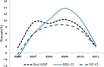
Yearly growth rates of BDL-CI, IIF-CI and real GDP.
timeliness and accuracy of economic activity estimates in Lebanon, we design two new indexes for the Lebanese economy: a coincident (WB-CI) and a leading (WB-LI) index. This study builds upon features from the empirical literature on coincident and leading indices such as Moore and Shiskin (1967), Stock and Watson (1989), Chauvet (1998), Mariano and Murasawa (2002), Issler and Vahid (2006), Pereira (2012) and Issler et al. (2013).
In this paper we add to the literature two main contributions. First, we improve on the NBER-Conference Board approach (Conference Board 2014) by employing a minimization technique to ameliorate the statistical properties of coincident and leading indexes. We do so by calibrating the weights assigned to each variable so that the yearly growth rate of the constructed index (Coincident or Leading) converges to the actual growth rate of the reference variable (in our case GDP) at any point in time. Second, we develop for the first time a leading index for the Lebanese economy that can be used to (i) detect early signs of turning points in economic activity and (ii) forecast GDP growth during the next 12 months.
The rest of this paper is structured as follows. Section 2 presents a brief historical overview of coincident and leading indexes. Section 3 describes the methodologies used to construct the WB-CI and WB-LI. Section 4 presents the results while Section 5 discusses some policy implications derived from these newly developed indexes. Finally, Section 6 presents the caveats and limitations of the indexes and Section 7 concludes.
2 Literature Review
Knowing the current and the expected state of the economy is of foremost importance for businesses, policymakers and investors. Depending on the quality of statistics in a given country, two distinct methodologies have been used to develop coincident and leading indexes: (i) the National Bureau of Economic Research (NBER) and/or Conference Board (CB) methodology and (ii) the Stock and Watson (1989) methodology (hereafter denoted by SW). The NBER-CB approach is a non-econometric technique, while the SW methodology is based on advanced statistical properties such as Dynamic Factor and Markov Switching models.
The idea of quantitatively monitoring a business cycle, which “commonly refers to co-movements in different forms of activity, not just fluctuations in GNP” (Stock and Watson 1989, 353), was first introduced in 1938 by a research team at the NBER. This team, which was led by Wesley Mitchell and Arthur Burns, examined the dynamics of some economic variables to see whether these changes lagged, led or coincided with changes observed in US business cycles. Twenty years later, Moore and Shiskin (1967) developed, for the first time and based on Burns and Mitchell’s (1946) research, a methodology to construct composite indexes of real economic activity. They designed “a scoring plan that has been developed to help in the evaluation and selection of indicators” (Moore and Shiskin 1967, 3). The scoring plan of each variable was based on (i) statistical adequacy, (ii) timeliness of publication, (iii) smoothness, (iv) economic significance, (v) historical business cycle conformity, and (vi) cyclical timing. This approach, which was adopted by the Conference Board in 1995 and developed later on, is, however, subject to some criticism. First, many econometricians argued that the selected variables were subjectively chosen without any econometric foundation (Marcellino 2005). This is what Koopmans (1947) described as a “measurement without theory”. Second, and as argued by Chauvet (1998) indexes constructed with this methodology are constantly revised ex-post and since revisions can be significant in certain cases, real-time assessment of the business cycle may be severely impacted.
In a first attempt to respond to these criticisms, Stock and Watson (1989) developed an econometric model to construct new coincident and leading indexes for the U.S. economy. In their method, the coincident indicator (or Index) is represented by an unobserved reference cycle representing what they referred to as the “state of the economy”. The index is then measured using a Dynamic Factor model, where the parameters of the series [5] forming the index are estimated using Maximum Likelihood and Kalman Filter methods. In addition, they developed a leading indicator that forecasts the growth rate of the coincident index over the next six months, using a set of variables [6] in a Vector Autoregressive model (VAR). However, the SW approach failed to anticipate the U.S. recession in 1990–1991 because it assumed that expansions and contractions are symmetric in terms of their impact on the economy. For that reason, and in order to account for the fact that recessions are more sudden and shorter than expansions, Chauvet (1998) improved on the SW methodology by capturing nonlinearities in the business cycle using the Markov Switching model as proposed by Hamilton (1989). Other noticeable scholars that tried to improve on the SW econometric methodology are Mariano and Murasawa (2002) who employed a mixed frequency model by adding quarterly real GDP data to the initial set of monthly indicators and Issler and Vahid (2006) who used canonical correlation analysis and an instrumental variable probit model to construct a coincident index of the US economy.
Historically, economic research in this area was focused on developed countries. However, as a result of the improvement in the quality and frequency of data, research examining business cycles in emerging countries increased in recent years. Consequently, economists deepened their understanding of the business cycle in many of these countries by developing coincident and/or leading indexes. For example, Saadi-Sedik and Mongardini (2003) employed a reduced form model of the SW methodology to construct coincident and leading indexes for the Jordanian economy from January 1996 to December 2002. More recently, Pereira (2012) constructed a quarterly coincident index for the Cape Verdean economy, from 2002 to 2010, using the NBER/CB approach, while Issler et al. (2013) designed coincident indexes for Argentina, Brazil, Chile, Colombia and Mexico. Finally, Dorsainvil (2014) designed a coincident index for the Haitian economy using the Principal Component Analysis approach.
Although the SW methodology provides a proper statistical framework, it can’t be applied in the Lebanese context due to the absence of long historical time-series. In particular, we only have yearly data for the Lebanese GDP from 2004 to 2011 which only gives us eight observations. Therefore, the law of large numbers, on which the relevant time-series econometric techniques depend, will be violated, hence decreasing the power of these models (higher probability of committing a Type II error). For that reason, we will use an improved NBER-CB approach which can be applied in countries that suffer from weak statistical systems (similar to Lebanon). This approach has the important advantage of being easy to construct, explain and analyze. These are valuable properties in constructing composite indexes aimed at a wide public.
3 Methodology
3.1 World Bank Coincident Index for Lebanon (WB-CI)
The construction of the WB-CI starts with the choice of a benchmark series, which in our case is the (recently revised) annual GDP series from 2005 [7] till 2011 as published by the Central Administration of Statistics (CAS) in October 2013. The next step is to select the corresponding variables that track as closely as possible the current dynamics of real GDP. The potential variables which satisfy this objective should be, above all, available with a monthly frequency and have a historical series that dates back to the earliest starting point of the new real GDP series published by CAS. This selection is crucial for computing the WB-CI, because if the set of potential variables does not cover all (or most of) the sectors of the Lebanese economy, then the WB-CI will not be a robust estimate of real GDP. Consequently, and in order to account for all the economic sectors, we refer to Lebanon’s GDP decomposition, presented in Table 1, and map each sector to a high-frequency variable that reflects its economic dynamics.
Lebanon’s GDP decomposition from the supply side.
| Agriculture and forestry | Industry | Services |
| Agriculture & forestry | Mining & quarrying | Wholesale & retail trade |
| Livestock & livestock products; fishing | Manufacturing of food products | Vehicle maintenance & repair |
| Beverages & tobacco manufacturing | Transport | |
| Textile & leather manufacturing | Hotels & restaurants | |
| Wood & paper manufacturing; printing | Information & communication | |
| Chemicals, rubber & plastics manufacturing | Financial services | |
| Non-metallic mineral manufacturing | Real estate | |
| Metal products, machinery & equipment | Professional services | |
| Other manufacturing | Administrative services | |
| Electricity | Public administration | |
| Water Supply & waste management | Education | |
| Construction | Health & social care | |
| Personal & community services |
The availability of sufficiently long time series is a major constraint in Lebanon. As a result, a relatively small number of variables exist to proxy for economic activity, [8] and many variables used in the literature to develop coincident indexes are not available in the case of Lebanon such as real personal income less transfers and the number of employees on non-agricultural payrolls. According to Anguyo (2011), the former captures consumers’ aggregate spending behavior while changes in the latter reflect net hiring in the economy.
3.1.1 Existing Data and Potential Variables for the WB-CI
A set of twenty potential variables, capturing the dynamics of most sectors of the Lebanese economy, was included in the construction of the WB-CI. The rationale for selecting each of these variables, listed with their corresponding sources in Table 6 in the Appendix, is the following:
The dynamics of the wholesale & retail trade sector, which is the main sector of the Lebanese economy, representing 14.8 % of GDP in 2011, are captured using cleared checks obtained from BdL and VAT revenues published in the public finance monitor of the ministry of finance.
The real estate sector, the second biggest sector of the Lebanese economy representing 13.8 % of GDP in 2011 is proxied using (i) real estate registration fees and (ii) tax on property. Data for both variables are also obtained from the public finance monitor published by the ministry of finance.
The public administration services sector is the third biggest sector of the economy representing 9.6 % of GDP in 2011. For activities in this sector, we use the primary spending (total spending minus interest payments) of the central government as a proxy.
The financial sector, representing 7.3 % of GDP in 2011, is measured using M3, lending to the private sector and non-resident private sector deposits, while the construction sector, which constituted 4.5 % of GDP in 2011, is captured using cement deliveries and construction permits. Data for both variables are obtained from BdL.
Due to the scarcity of variables reflecting the activity of the industrial and agricultural sectors, which represented respectively 3.8 and 13.4 % of GDP in 2011, these sectors are measured using net exports of goods (excluding energy imports) calculated based on data provided by the Lebanese customs.
Finally, the information and communication, tobacco manufacturing, administrative services, transport, electricity and hotels and restaurants sectors are captured using transfer from the telecom surplus, tobacco excise, administrative fees and charges, private car registration fees, imports of energy and tourist arrivals, respectively. [9] In addition, current economic index, current personal income index and the current security index were used as proxies for consumer sentiment.
3.1.2 Steps Followed to Construct the WB-CI
The WB-CI we construct is based on a methodology that is similar, but not identical, to the NBER-CB approach. The main difference resides in the choice of weights. In contrast to the latter methodology, which computes the weights assigned to each variable as the inverse of its respective standard deviation, the weights in the WB-CI are calibrated in order to minimize the difference between the average yearly growth rate of the coincident index and the actual GDP growth rate as published by CAS. In other words, the weights are selected such that the growth rate of the WB-CI is as close as possible to the GDP growth rate during the same year. In particular, our methodology is based on nine distinct steps. In what follows,
The X-12-ARIMA technique with a multiplicative decomposition is used to remove the seasonal trend from all the variables
In order to measure the real economic activity, all the variables that are in monetary terms are deflated by the Consumer Price Index (CPI) published by the Consultation and Research Institute (CRI) [11] with December 2006 as the base period/month.
Fiscal variables exhibit unusual volatility at a monthly frequency. To eliminate this “noise” we smooth these series using six months moving averages.
Then, the month-to-month symmetric percentage change is calculated. [12] If the variable
[1]In any other case, the following symmetric percentage change formula is applied.
[2]Before proceeding, let
Afterwards, (preliminary) random weights
Using steps 4 and 5 the growth rate,
[3]Next, the growth rates of all the variables are summed in order to get the month-to-month growth rate,
[4]Assuming that the base year of the WB-CI is the first period (i. e.
[5]
After following the above steps and calibrating the model using the minimization problems in eqs [6] and [7], the WB-CI is constructed from December 2004 to December 2011 (85 observations). Table 2 shows that the WB-CI is a weighted average of twelve variables with VAT revenues, lending to the private sector, primary spending, administrative fees and charges, and M3 contributing the most, while the other eight variables (not shown in Table 2) were apportioned a zero weight.
Variables forming the WB-CI.
| Variable | Weight (%) |
| Net exports of goods without energy products* | 0.4 |
| Taxes on real-estate | 0.7 |
| Tourist arrivals | 3.4 |
| Non-resident private sector deposits | 3.7 |
| Tobacco excise | 6.1 |
| Cleared checks | 6.2 |
| Cement deliveries | 6.3 |
| VAT revenues | 13.0 |
| Lending to the private sector | 13.9 |
| Primary spending | 14.7 |
| Administrative fees and charges | 15.0 |
| M3 | 16.6 |
| Total | 100.0 |
3.2. World Bank Leading Index of Lebanon (WB-LI)
In a turbulent and volatile environment like Lebanon, a high-frequency leading index is a natural complement to a coincident index. A leading index for the Lebanese economy (WB-LI) would help to (i) detect early signs of turning points in the economic activity and (ii) forecast GDP growth during the next 12 months. To the best of our knowledge, the designed WB-LI would be the only publicly available leading index for the Lebanese economy.
3.2.1 Existing Data and Potential Variables for the WB-LI
The initial steps in constructing the WB-LI are to (i) choose an appropriate reference series and to (ii) determine the relevant components of the WB-LI. We will use the developed WB-CI as the benchmark series because by construction it follows the business cycle of the Lebanese economy very closely. We should note that potential variables that satisfy at least one of the following two conditions can be used in the construction of the WB-LI. The first condition is economic significance, implying that a certain variable has “expectational components that would (under some economic theory) respond rapidly to some shocks to the economy” (Stock and Watson 1989, 365). The second is statistical relevance which means that the correlation coefficient between a certain variable at time
While the choice of variables based on the statistical relevance principle depends, solely, on having a correlation coefficient larger than 0.5, the variables that we selected according to the economic significance criteria would warrant a greater analysis. For example, the future economic index reflects the expectations of individuals regarding the future economic environment. On the other hand, an increase in personnel costs [13] implies that workers have more money to save and spend today. Given the high Lebanese interest rates, this implies that a rational person would prefer to save today, earn a high return and then consume in the future. Moreover, higher capital spending suggests that the government is planning to boost economic activity in the future through investing in capital projects today. Meanwhile, freight incoming at the port of Beirut is a leading retail trade indicator as businesses and industrialists import more goods in the present when expecting an improvement in the general business environment in the future. The stock index reflects investors’ appetite to invest in the future while the EMBIG spread captures investors’ confidence in sovereign bonds. In addition, the dollarization rate and the spread between local and interest rates can both be considered leading indicators as the former is a proxy for the confidence in the local currency while the latter is a major determinant of future deposit inflows at commercial banks. Finally, an increase in construction permits suggests that investors and contractors expect a pickup in the real estate sector in the long run as it takes several years to construct a building.
Economic significance and statistical relevance of the potential variables of the WB-LI.
| Variable | Statistical Relevance* | Economic Significance** |
| Consumer Confidence Index | × (+0.32) | ✓ |
| Cement Deliveries | ✓(+0.72) | × |
| EMBIG Spread | ✓(+0.79) | ✓ |
| Custom Revenues | ✓(+0.58) | ✓ |
| Airport Arrivals | ✓(+0.84) | × |
| Freight Incoming at the Port of Beirut | × (+0.37) | ✓ |
| Spread between local and Libor interest rate | ✓(+0.89) | ✓ |
| Lending to the Private Sector | ✓(+0.86) | ✓ |
| Personnel Cost | × (+0.47) | ✓ |
| Capital Expenditures | × (–0.07) | ✓ |
| Change in Dollarization Rate | × (–0.04) | ✓ |
| Public Debt | ✓ (+0.92) | ✓ |
| Blom Stock Index | × (–0.06) | ✓ |
| Industrial Exports | ✓ (+0.69) | × |
| Construction Permits | × (+0.49) | ✓ |
| Construction in Progress | × (–0.02) | ✓ |
| Future Economic Index | × (–0.08) | ✓ |
3.2.2 Steps Followed to Construct the WB-LI
To develop the WB-LI, we use the same methodology adopted for constructing the WB-CI with the exception of a different minimization problem (step 9). In particular, the weights are calibrated in order to minimize the difference between the growth rate of the leading index at time
The adjustment in the methodology and the ensuing calibration generated the WB-LI from December 2006 to December 2012 (73 observations). As shown in Table 4, the constructed WB-LI consists of monthly observations for nine variables (real, external, monetary and fiscal) while the other eight variables (not shown in Table 4) were apportioned a 0 weight as a result of the minimization.
Variables forming the WB-LI.
| Variable | Weight (%) |
| EMBIG spread | 0.09 |
| Custom revenues | 0.47 |
| Spread between local and Libor interest rate | 5.05 |
| Capital expenditures | 5.26 |
| Lending to private Sector | 10.85 |
| Airport arrivals | 15.46 |
| Cement deliveries | 15.66 |
| Freight incoming at port of Beirut | 22.41 |
| Personnel costs | 24.75 |
| Total | 100.00 |
4 Results of the WB-CI and the WB-LI
Our results indicate that the designed WB-CI measures the economic activity in Lebanon very accurately. [15] The criteria used to assess the effectiveness of the WB-CI in monitoring the Lebanese economic activity is based on calculating the absolute value of the error between the yearly growth rate of the WB-CI and the actual (realized) annual GDP growth rate. When this error tends, on average, to 0 and its standard deviation converges to 0 this implies that the WB-CI accurately reflects the dynamics of the Lebanese real economy. As reported in Table 5, the average error and the standard deviation between 2006 and 2011 were both equal to 0.0 %. This compares favorably to both the BdL and the IIF coincident indexes. For the BdL-CI (IIF-CI), the average growth rate was 2.37 (1.53) % and the standard deviation was 1.29 (1.14) % during the same period. Consequently, the WB-CI is a reliable measure of the current state of the Lebanese economy.
Error between GDP growth and each of WB-CI, BDL-CI and IIF-CI.
| WB-CI Growth (%) | BDL-CI Growth (%) | IIF-CI Growth (%) | GDP Growth (%) | Absolute value of error between WB-CI Growth and GDP Growth (%) | Absolute value of error between BDL-CI Growth and GDP Growth (%) | Absolute value of error between IIF-CI Growth and GDP Growth (%) | |
| 2006 | 1.6 | −1.4 | −0.4 | 1.6 | 0.0 | 3.0 | 2.0 |
| 2007 | 9.4 | 5.8 | 5.9 | 9.4 | 0.0 | 3.6 | 3.5 |
| 2008 | 9.1 | 10.2 | 8.2 | 9.1 | 0.0 | 1.1 | 0.9 |
| 2009 | 10.3 | 13.8 | 8.7 | 10.3 | 0.0 | 3.5 | 1.6 |
| 2010 | 8.0 | 10.5 | 7.0 | 8.0 | 0.0 | 2.5 | 1.0 |
| 2011 | 2.0 | 2.5 | 1.8 | 2.0 | 0.0 | 0.5 | 0.2 |
| 2012e | 2.2 | ||||||
| 2013e | 0.8 | ||||||
| 2014e | 1.2 | ||||||
| Memorandum items: | |||||||
| Average of Error (2006–2011) | 0.0 | 2.4 | 1.5 | ||||
| Standard deviation of Error (2006–2011) | 0.0 | 1.3 | 1.1 | ||||
| Correlation Coefficient | 1.0 | 0.9 | 1.0 | ||||
The one-year ahead forecasting performance of the constructed WB-LI is encouraging.
[16] As illustrated in Figure 2, the yearly average growth rate of the WB-LI leads the yearly growth rate of the WB-CI by a year. Furthermore, Figure 3 shows that the yearly growth rate of the leading indicator at time
The WB-LI is a good tool to detect turning points in the economy….
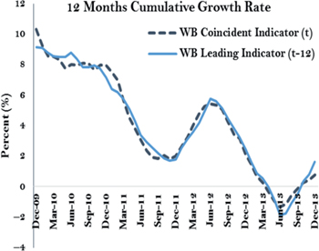
… and forecast economic growth in the short-run.
To illustrate the importance of having timely and accurate economic data, it is instructive to look at the monetary policy implications of the (new) WB-CI versus that of the existing BdL-CI. As detailed below, the latest reading from the BdL-CI points to a constant growth in economic activity. The WB-CI, however, is showing an economy that is accelerating. The growth rate of the BdL-CI was constant at 3.2 % between 2013 and 2014, suggesting that the Lebanese economy grew at the same pace. In contrast, the WB-CI showed that the economy grew by 1.2 % in 2014 compared to 0.8 % during 2013, reflecting an acceleration in economic activity. A sustained period with such diverging trends would result in sharply different monetary policy decisions.
5 Some Policy Implications
In this section, we examine the impact of unexpected changes in macroeconomic variables on economic growth using the WB-CI decomposition. We employ a Vector Autoregressive (VAR) model to examine the relationship between the variables forming the WB-CI and real GDP growth as proxied by the growth rate of the WB-CI itself. A necessary condition for VAR models to be econometrically valid is the stationarity of variables. Table 10, in the Appendix, shows that the log differences of WB-CI, tobacco excise (TE), cement deliveries (CD), VAT revenues (VAT), tourist arrivals (TA), taxes on real estate (TR), money supply (M3), lending to the private sector (LP), administrative fees and charges (AC), non-resident deposits (NRD), primary spending (PS), and cleared checks (CC) are found to be stationary at the 10 % level.
[17] Let
where
We proceed to generate, the Impulse Response Functions (IRFs) for the VAR(k) model. The results of the IRFs, illustrated in Figure A1 (in the Appendix), trace the response of real economic activity (proxied by the WB-CI) to one standard deviation shocks in each variable
In order to examine causality between the
Finally, and based on the significant IRFs and the Granger causality tests, the economy would be expected to grow, as show in Table 13, by 0.03, 0.2, 0.21, 0.21 and 0.32 percentage points next year if we observe a one percentage point increase in cement deliveries, cleared checks, tobacco excise, administrative fees and charges and VAT revenues respectively this year.
6 Caveats and Limitations
While the newly developed indexes reveal promising statistical properties in terms of estimating and forecasting real economic activity in Lebanon, analysts and policy makers should be aware of the following limitations of the model when interpreting the results:
First, not all the sectors of the economy were adequately represented in the pool of potential variables due to data limitations. Most notably, good proxy variables were not available to accurately account for the agriculture and industry sectors, which combined accounted for 18.6 % of GDP in 2011.
Second, due to data limitations we deflated all the monetary variables into real terms using the CRI consumer price index that only account for the price dynamics in the greater capital area (greater Beirut). However, the Central Administration of Statistics (CAS) has recently (March, 2014) rebased Lebanon’s inflation data to December 2013 and now provides (i) a much more comprehensive breakdown of prices (prices for rent are now collected on a monthly basis) and (ii) an updated weighting scheme to the inflation basket. As a result, this improved CAS CPI series could be preferable to the one currently used, once the old (2007) CPI index is rebased to the new (2014) index in order to have a continuous and comparable CPI series.
Third, the lag period of the WB-CI and the WB-LI appeared to be larger (4–5 months) than initially expected due to the infrequent and lagged release of the fiscal data from the ministry of finance.
Fourth, and as illustrated in figure 4, economic activity in Lebanon is highly volatile and subject to frequent exogenous shocks of political and security nature. However, this volatility is not captured by the WB-LI as it is hard to predict sudden changes in the political and/or security conditions. As a result, analysts should take into account any recent political developments rather than interpreting the results mechanically.
Fifth and most importantly, the yearly growth rate of the newly constructed indexes were only tested against six actual GDP growth observations (2006–2011) because longer time series were not available. As a result, some non-negligible margin of error is expected to remain in the estimates and results. In order, to improve the efficiency of the estimates, the model will be recalibrated whenever new national accounts data are published by CAS.
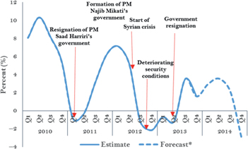
Estimated quarterly growth based on WB-CI and WB-LI (yoy).
7 Conclusion
This paper presents a new coincident index (WB-CI) and a 12-months leading index (WB-LI) for the Lebanese economy. These indexes, which can be used as monthly proxies for the evolution of real GDP, were constructed using an improved methodology based on the NBER-CB approach.
Notwithstanding the relatively small sample period, the results reveal promising statistical properties that should make these new indications valuable coincident and leading (one-year ahead) indexes for monitoring the Lebanese economy. However, given limitations on the length of time series in Lebanon, the accuracy and reliability of these indexes in tracking the business cycle of the Lebanese economy is expected to improve over time as more data points become available. To take into account the statistical value of these new data points, both indexes will be re-estimated periodically. It is therefore likely that the composition of the WB-CI and the WB-LI will change in the coming years and become more stable as actual GDP series from national authorities are published. Furthermore, and rather than analyzing the results of these indexes mechanically, analysts should incorporate into their assessment of economic activity historical, political and cultural factors that do not easily lend themselves to quantification.
Finally, this new approach of adding a minimization problem to the original NEBR-CB methodology may provide a useful roadmap to analyze business cycles in countries that have weak economic statistics.
Acknowledgments
The author would like to thank Eric le Borgne, Ibrahim Jamali, Wissam Harake, Lionel Roger and two anonymous referees for their comments and suggestions. The auhtors would like also to thank participants at the World Bank seminar and staff from Banque du Liban and the IMF for their stimulating discussions.
Appendix
Potential variables for inclusion in the WB-CI.
| Variable | Unit | Source |
| Administrative fees and charges | LBP bln | Ministry of Finance |
| Car Excise | LBP bln | Ministry of Finance |
| Cement Deliveries | thousands of tons | Banque du Liban |
| Cleared checks | LBP bln | Banque du Liban |
| Construction Permits | m2 | Banque du Liban |
| Current Economic Index | Index | ARA marketing research and consultancy |
| Current Personal Income Index | Index | ARA marketing research and consultancy |
| Current Security Index | Index | ARA marketing research and consultancy |
| Energy Imports | LBP bln | Lebanese Customs |
| Exports of Goods | LBP bln | Lebanese Customs |
| Imports of Goods without energy products | LBP bln | Lebanese Customs |
| Lending to the private sector | LBP bln | Banque du Liban |
| M3 | LBP bln | Banque du Liban |
| Primary spending | LBP bln | Ministry of Finance |
| Private car registration | LBP bln | Ministry of Finance |
| Non-Resident Private sector deposits | LBP bln | Banque du Liban |
| Taxes on real-estate* | LBP bln | Ministry of Finance |
| Tobacco Excise | LBP bln | Ministry of Finance |
| Tourist arrivals | number | Ministry of Tourism |
| VAT revenues | LBP bln | Ministry of Finance |
Potential variables for inclusion in the WB-LI.
| Variable | Unit | Source |
| Consumer confidence index | Index | ARA Research & Consultancy |
| Cement deliveries | thousand tons | Banque du Liban |
| EMBIG spread | bps | JP Morgan; WB staff calculations |
| Custom revenues | LBP bln | Ministry of Finance |
| Airport arrivals | number | Banque du Liban |
| Freight incoming at the port of Beirut | tons | Banque du Liban |
| Spread between local and Libor interest rate | bps | Banque du Liban; WB staff calculations |
| Lending to private sector | LBP bln | Banque du Liban |
| Personnel costs | LBP bln | Ministry of Finance |
| Capital expenditures | LBP bln | Ministry of Finance |
| Change in dollarization rate | bps | BDL; WB staff calculations |
| Public debt | LBP bln | Banque du Liban |
| Blom stock index | Index | BLOM Bank |
| Industrial exports | mln USD | Ministry of Industry |
| Construction permits | m2 | Banque du Liban |
| Construction in progress | LBP bln | Ministry of Finance |
| Future Economic Index | Index | ARA Research & Consultancy |
WB-CI data.
| Date | Value | Date | Value | Date | Value |
| WB-CI (Dec-2004=100) | |||||
| Jan-05 | 98.1 | Jan-08 | 112.8 | Jan-11 | 141.7 |
| Feb-05 | 93.7 | Feb-08 | 116.1 | Feb-11 | 141.8 |
| Mar-05 | 93.6 | Mar-08 | 115.5 | Mar-11 | 142.2 |
| Apr-05 | 95.2 | Apr-08 | 115.2 | Apr-11 | 144.4 |
| May-05 | 97.0 | May-08 | 116.1 | May-11 | 144.6 |
| Jun-05 | 101.4 | Jun-08 | 121.6 | Jun-11 | 147.8 |
| Jul-05 | 103.0 | Jul-08 | 122.6 | Jul-11 | 149.0 |
| Aug-05 | 104.6 | Aug-08 | 126.1 | Aug-11 | 147.4 |
| Sep-05 | 107.2 | Sep-08 | 124.1 | Sep-11 | 152.3 |
| Oct-05 | 101.7 | Oct-08 | 125.8 | Oct-11 | 153.2 |
| Nov-05 | 100.8 | Nov-08 | 130.1 | Nov-11 | 148.7 |
| Dec-05 | 104.4 | Dec-08 | 130.6 | Dec-11 | 156.0 |
| Jan-06 | 103.6 | Jan-09 | 134.1 | Jan-12 | 152.2 |
| Feb-06 | 108.7 | Feb-09 | 133.0 | Feb-12 | 153.0 |
| Mar-06 | 110.4 | Mar-09 | 130.3 | Mar-12 | 150.9 |
| Apr-06 | 114.0 | Apr-09 | 131.6 | Apr-12 | 153.9 |
| May-06 | 114.8 | May-09 | 133.9 | May-12 | 153.2 |
| Jun-06 | 109.8 | Jun-09 | 131.5 | Jun-12 | 152.5 |
| Jul-06 | 77.0 | Jul-09 | 134.8 | Jul-12 | 149.3 |
| Aug-06 | 78.8 | Aug-09 | 134.1 | Aug-12 | 145.4 |
| Sep-06 | 99.3 | Sep-09 | 133.2 | Sep-12 | 148.4 |
| Oct-06 | 97.1 | Oct-09 | 137.5 | Oct-12 | 148.7 |
| Nov-06 | 108.6 | Nov-09 | 134.2 | Nov-12 | 149.1 |
| Dec-06 | 106.5 | Dec-09 | 137.2 | Dec-12 | 150.2 |
| Jan-07 | 105.3 | Jan-10 | 141.4 | Jan-13 | 150.6 |
| Feb-07 | 110.4 | Feb-10 | 141.6 | Feb-13 | 150.1 |
| Mar-07 | 111.1 | Mar-10 | 146.5 | Mar-13 | 152.2 |
| Apr-07 | 110.8 | Apr-10 | 147.0 | Apr-13 | 152.6 |
| May-07 | 111.9 | May-10 | 144.9 | May-13 | 151.4 |
| Jun-07 | 110.5 | Jun-10 | 146.1 | Jun-13 | 150.1 |
| Jul-07 | 111.1 | Jul-10 | 147.5 | Jul-13 | 152.9 |
| Aug-07 | 112.9 | Aug-10 | 144.3 | Aug-13 | 154.5 |
| Sep-07 | 113.3 | Sep-10 | 143.1 | Sep-13 | 151.3 |
| Oct-07 | 110.2 | Oct-10 | 143.4 | Oct-13 | 151.5 |
| Nov-07 | 113.9 | Nov-10 | 143.4 | Nov-13 | 153.3 |
| Dec-07 | 112.4 | Dec-10 | 144.3 | Dec-13 | 150.3 |
WB-LI data.
| Date | Value | Date | Value | Date | Value | Date | Value |
| WB-LI (Dec-2006 = 100) | |||||||
| Jan-07 | 101.7 | Jan-09 | 119.8 | Jan-11 | 129.9 | Jan-13 | 132.0 |
| Feb-07 | 106.2 | Feb-09 | 118.0 | Feb-11 | 128.5 | Feb-13 | 134.0 |
| Mar-07 | 105.5 | Mar-09 | 119.7 | Mar-11 | 127.2 | Mar-13 | 129.3 |
| Apr-07 | 104.5 | Apr-09 | 121.1 | Apr-11 | 128.3 | Apr-13 | 129.2 |
| May-07 | 104.8 | May-09 | 122.4 | May-11 | 129.9 | May-13 | 130.3 |
| Jun-07 | 106.6 | Jun-09 | 122.8 | Jun-11 | 129.5 | Jun-13 | 131.0 |
| Jul-07 | 101.7 | Jul-09 | 122.7 | Jul-11 | 125.4 | Jul-13 | 132.5 |
| Aug-07 | 98.7 | Aug-09 | 121.4 | Aug-11 | 122.1 | Aug-13 | 132.5 |
| Sep-07 | 100.9 | Sep-09 | 121.3 | Sep-11 | 124.1 | Sep-13 | 130.5 |
| Oct-07 | 104.6 | Oct-09 | 121.5 | Oct-11 | 123.3 | Oct-13 | 129.5 |
| Nov-07 | 103.7 | Nov-09 | 122.7 | Nov-11 | 127.3 | Nov-13 | 128.2 |
| Dec-07 | 107.6 | Dec-09 | 123.9 | Dec-11 | 124.8 | Dec-13 | 127.1 |
| Jan-08 | 110.5 | Jan-10 | 119.4 | Jan-12 | 127.8 | ||
| Feb-08 | 114.0 | Feb-10 | 119.3 | Feb-12 | 126.6 | ||
| Mar-08 | 113.8 | Mar-10 | 119.9 | Mar-12 | 129.7 | ||
| Apr-08 | 112.8 | Apr-10 | 120.4 | Apr-12 | 128.0 | ||
| May-08 | 113.4 | May-10 | 120.5 | May-12 | 126.4 | ||
| Jun-08 | 112.5 | Jun-10 | 120.7 | Jun-12 | 122.7 | ||
| Jul-08 | 114.2 | Jul-10 | 125.1 | Jul-12 | 127.8 | ||
| Aug-08 | 112.9 | Aug-10 | 125.0 | Aug-12 | 129.5 | ||
| Sep-08 | 110.6 | Sep-10 | 127.6 | Sep-12 | 129.9 | ||
| Oct-08 | 112.0 | Oct-10 | 126.7 | Oct-12 | 132.2 | ||
| Nov-08 | 114.0 | Nov-10 | 129.3 | Nov-12 | 132.4 | ||
| Dec-08 | 119.5 | Dec-10 | 130.2 | Dec-12 | 132.1 | ||
Unit Root test results.
| Variable | ADF-Test (p-value) |
| ld_WB_CI | 1.055e-017 *** |
| ld_Tobacco_Excise | 2.7e-005 *** |
| ld_Cement_Deliveries | 1.835e-023*** |
| ld_VAT_revenues | 6.573e-014 *** |
| ld_Tourists_Arrivals | 1.068e-017*** |
| ld_Real_estate_tax | 9.575e-005*** |
| ld_M3 | 0.07188* |
| ld_Lending_private | 0.01208** |
| ld_Administrative_Charges | 5.18e-009*** |
| ld_non-resid Deposits | 4.598e-012*** |
| ld_Primary_Spending | 0.009343*** |
| ld_Cleared_Checks | 2.29e-016*** |
Contribution of a shock in variable k’ on the variance decomposition of WB-CI (%).
| Month | ld_M3 | ld_TA | ld_TE | ld_CC | ld_CD | ld_AC | ld_VAT |
| M1 | 19.6 | 30.7 | 4.7 | 33.1 | 29.1 | 38.8 | 8.6 |
| M2 | 19.6 | 31.6 | 27.7 | 35.0 | 28.8 | 38.6 | 83.1 |
| M3 | 17.2 | 31.8 | 36.6 | 32.1 | 27.5 | 39.1 | 83.3 |
| M4 | 17.1 | 31.8 | 38.2 | 33.6 | 27.9 | 38.1 | 85.5 |
| M5 | 18.4 | 32.4 | 36.7 | 32.2 | 28.5 | 43.1 | 83.2 |
| M6 | 18.4 | 32.3 | 36.5 | 32.2 | 28.9 | 43.2 | 83.5 |
| M7 | 19.0 | 32.3 | 36.7 | 32.4 | 28.8 | 43.9 | 83.5 |
| M8 | 23.0 | 32.3 | 36.7 | 32.4 | 28.7 | 43.3 | 83.7 |
| M9 | 23.1 | 32.3 | 36.5 | 32.1 | 33.4 | 43.3 | 83.5 |
| M10 | 23.7 | 32.3 | 36.5 | 32.3 | 33.1 | 43.1 | 83.5 |
| M11 | 23.7 | 32.3 | 36.5 | 32.4 | 33.7 | 43.1 | 83.5 |
| M12 | 23.9 | 32.3 | 36.4 | 32.4 | 33.4 | 43.1 | 83.5 |
| M13 | 23.9 | 32.3 | 36.4 | 32.5 | 33.1 | 43.2 | 83.5 |
| M14 | 24.5 | 32.3 | 36.4 | 32.6 | 33.0 | 43.2 | 83.5 |
| M15 | 24.7 | 32.3 | 36.5 | 32.6 | 32.9 | 43.2 | 83.5 |
| M16 | 24.6 | 32.3 | 36.4 | 32.6 | 33.0 | 43.2 | 83.5 |
| M17 | 24.6 | 32.3 | 36.4 | 32.6 | 33.0 | 43.2 | 83.5 |
| M18 | 24.7 | 32.3 | 36.4 | 32.6 | 33.4 | 43.2 | 83.5 |
| M19 | 24.7 | 32.3 | 36.4 | 32.6 | 33.2 | 43.2 | 83.5 |
| M20 | 24.8 | 32.3 | 36.4 | 32.6 | 33.2 | 43.2 | 83.5 |
| M21 | 24.9 | 32.3 | 36.4 | 32.6 | 33.1 | 43.2 | 83.5 |
| M22 | 25.0 | 32.3 | 36.4 | 32.6 | 33.1 | 43.2 | 83.5 |
| M23 | 25.0 | 32.3 | 36.4 | 32.6 | 33.1 | 43.2 | 83.5 |
| M24 | 25.0 | 32.3 | 36.4 | 32.6 | 33.1 | 43.2 | 83.5 |
Granger causality test.
| Null Hypothesis: No Granger Causality | p-value | No. of Lags (AIC) |
| M3 and WB-CI: | ||
| M3 Granger causes WB-CI | 0.128 | 7 |
| WB-CI Granger causes M3 | 0.0006*** | 7 |
| TA and WB-CI: | ||
| TA Granger causes WB-CI | 0.246 | 3 |
| WB-CI Granger causes TA | 0.0000*** | 3 |
| TE and WB-CI: | ||
| TE Granger causes WB-CI | 0.0000*** | 5 |
| WB-CI Granger causes TE | 0.0000*** | 5 |
| CC and WB-CI: | ||
| CC Granger causes WB-CI | 0.015** | 5 |
| WB-CI Granger causes CC | 0.0000*** | 5 |
| CD and WB-CI: | ||
| CD Granger causes WB-CI | 0.0003*** | 8 |
| WB-CI Granger causes CD | 0.0000*** | 8 |
| AC and WB-CI: | ||
| AC Granger causes WB-CI | 0.0000*** | 4 |
| WB-CI Granger causes AC | 0.0326** | 4 |
| VAT and WB-CI: | ||
| VAT Granger causes WB-CI | 0.0000*** | 4 |
| WB-CI Granger causes VAT | 0.0000*** | 4 |
Impact of a one percentage point shock on the WB-CI growth rate.
| Value in 2012 (LL bln) | 1 pp shock in Dec 2012 (LL bln) | Change in WB-CI Growth (%) | ||
| 2013 | 2014 | |||
| CD | 5299 | 53 | 0.03 | –0.01 |
| VAT | 2434 | 24 | 0.32 | 0.02 |
| CC | 79159 | 792 | 0.15 | 0.00 |
| TE | 382 | 4 | 0.21 | 0.02 |
| AC | 434 | 4 | 0.21 | −0.01 |
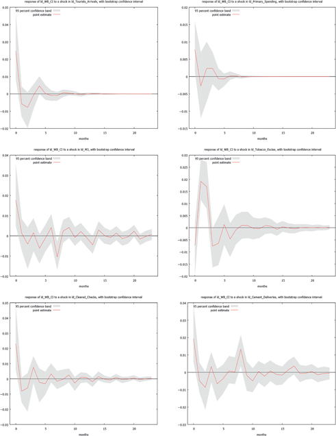
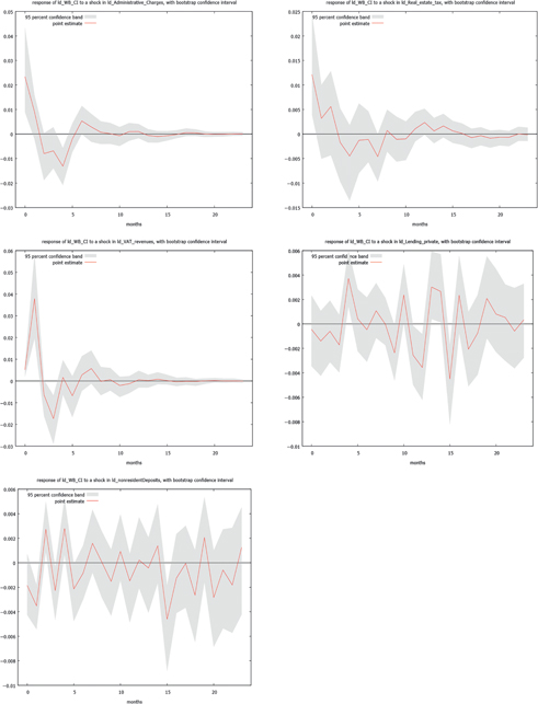
Impulse response functions of WB-CI to each k variable.
References
Anguyo, F. 2011. A Model to Estimate a Composite Indicator of Economic Activity (CIEA) for Uganda. Research Department: Bank of Uganda.Suche in Google Scholar
Burns, A., and W. Mitchell. 1946. “Measuring Business Cycles.” National Bureau of Economic Research.Suche in Google Scholar
Central Administration of Statistics. 2013, July. Retrieved from CAS: http://www.cas.gov.lb/images/PDFs/National%20Accounts/CAS_Lebanon_National_Accounts_2011_Comments_and_tables.pdf.Suche in Google Scholar
Chauvet, M. 1998. “An Econometric Characterization of Business Cycle Dynamics with Factor Structure and Regime Switching.” International Economic Review 39 (4):969–96.10.2307/2527348Suche in Google Scholar
Conference Board. 2014, March. Calculating the Composite Indexes. https://www.conference-board.org/data/bci/index.cfm?id=2154.Suche in Google Scholar
Dorsainvil, K. 2014. “Business Cycle in the Haitian Economy.” The Journal of Developing Areas 48 (3):65–75.10.1353/jda.2014.0056Suche in Google Scholar
Granger, C. 1969. “Investigating Causal Relations by Econometric Models and Cross-Spectral Methods.” Econometrica 37 (3):424–38.10.2307/1912791Suche in Google Scholar
Hamilton, J. 1989. “A New Approach to the Economic Analysis of Nonstationary Time Series and the Business Cycle.” Econometrica 57 (2):357–84.10.2307/1912559Suche in Google Scholar
IMF. 2012. Lebanon: 2011 Article IV Consultation, IMF Country Report No. 12/39. Washington, DC.Suche in Google Scholar
Iradian, G., and N. Zouk. 2010. Lebanon: New Estimates Reveal Exceptional Growth. Washington, DC: International Institute of Finance.Suche in Google Scholar
Issler, J., and F. Vahid. 2006. “The Missing Link: Using the NBER Recession Indicator to Construct Coincident and Leading Indices of Economic Activity.” Journal of Econometrics 132:281–303.10.1016/j.jeconom.2005.01.031Suche in Google Scholar
Issler, J., H. Notini, C. Rodrigues, and A. Soares. 2013. “Constructing Coincident Indices of Economic Activity for the Latin American Economy.” Revista Brasileira De Economia 67 (1/):67–96.10.1590/S0034-71402013000100004Suche in Google Scholar
Jad, S. S. 2011. “The Use of Surveys to Measure Sentiment and Expected Behaviour of Key Sectors in the Economy: Evidence From the Business Survey Conducted by the Central Bank of Lebanon.” IFC Bulletin 34:248–77.Suche in Google Scholar
Koopmans, T. 1947. “Measurement Without Theory.” The Review of Economics and Statistics XXIX (3):161–79.10.2307/1928627Suche in Google Scholar
Marcellino, M. 2005. Leading Indicators: What Have We Learned? CEPR Discussion Paper No. 4977.10.2139/ssrn.695721Suche in Google Scholar
Mariano, R., and Y. Murasawa. 2002. “A New Coincident Index of Business Cycles Based on Monthly and Quarterly Series.” Journal of Applied Econometrics 18 (4):427–43.10.1002/jae.695Suche in Google Scholar
Mongardini, J., and T. Saadi-Sedik. 2003. Estimating Indexes of Coincident and Leading Indicators: An Application to Jordan. IMF Working Paper, WP/03/170.Suche in Google Scholar
Moore, G., and J. Shiskin. 1967. Indicators of Business Expansions and Contractions. National Bureau of Economic, Occasional paper 103.Suche in Google Scholar
Pereira, E. 2012. “A Quarterly Coincident Indicator for the Cape Verdean Economy.” Banco De Cabo Verde. 13/2012.Suche in Google Scholar
Stock, J., and M. Watson. 1989. “New Indexes of Coincident and Leading Economic Indicators.” National Bureau of Economic Research Macroeconomics Annual 1989 4:351–409.10.1086/654119Suche in Google Scholar
©2015 by De Gruyter
Artikel in diesem Heft
- Frontmatter
- Research Articles
- Foreign Bank Entry in the Late Ottoman Empire: The Case of the Imperial Ottoman Bank
- Is Bigger Better for Egyptian Banks? An Efficiency Analysis of the Egyptian Banks during a Period of Reform 2000–2006
- Provisioning, Bank Behavior and Financial Crisis: Evidence from GCC Banks
- New Coincident and Leading Indexes for the Lebanese Economy