IUPAC/CITAC guide: interlaboratory comparison of categorical characteristics of a substance, material, or object (IUPAC Technical Report)
-
Ilya Kuselman

 ,
Tamar Gadrich
,
Francesca R. Pennecchi
,
D. Brynn Hibbert
,
Anastasia A. Semenova
and
Angelique Botha
,
Tamar Gadrich
,
Francesca R. Pennecchi
,
D. Brynn Hibbert
,
Anastasia A. Semenova
and
Angelique Botha

Abstract
This Guide is intended for harmonization of interlaboratory comparisons of categorical − nominal (qualitative, i.e., non-quantitative) and ordinal (semi-quantitative) − characteristics of a substance, material, or object. It provides guidance for application of relevant methods of mathematical statistics for design of such interlaboratory comparisons and analysis of the obtained data, when the methods developed for continuous quantitative values (e.g., ANOVA − analysis of variance) cannot be used without violation of their basic assumptions. The proposed approach employs recently-developed two-way nominal analysis of variation CATANOVA and two-way ordinal analysis of variation ORDANOVA. The Guide also addresses correlation between the categorical characteristics, as well as correlation between these characteristics and the chemical composition of the material or object. A multisensory quality index of a product, combining information on its categorical characteristics, is detailed. It allows for comparison of the quality of the same material produced by different producers. The examples provided in the Guide are from the fields of macroscopic examination of weld imperfections, comparison of odor intensity of drinking water, and comparison of sensory (ordinal) characteristics of a sausage. A corresponding calculation tool with an Excel spreadsheet including macros, and programs written in the R environment, are available in the specified references.
1 Introduction
Interlaboratory studies are widely used for estimation of proficiency/competence of calibration and testing (including chemical analytical and medical) laboratories in specific measurements, tests, calibrations, examinations, inspections or sampling; 1 for development of certified reference materials; 2 for validation of measurement and testing methods; 3 , 4 and for evaluation of calibration and measurement capabilities of national metrology institutes and designated institutes participating in key and supplementary comparisons. 5 When the reference value for the measurand is unknown, agreement (consistency) of the measured values obtained by the participating laboratories is investigated. 6 , 7 If suitable agreement is observed and outliers are absent or treated, the laboratory results may then be used for estimating (building) a consensus value of the measurand that is applicable in the absence of a known reference value. 8 , 9 , 10 The consensus value typically is an arithmetic mean of measured values, when their distribution is approximately symmetric and associated measurement uncertainties are approximately equal; a weighted mean of the values with weights depending on their measurement uncertainties; a Bayesian estimator; 11 , 12 or a robust estimator of a population mean. 1 , 13 When the reported measurement uncertainties do not sufficiently cover the actual differences between laboratory results, an interlaboratory “dark” uncertainty component, not considered by the laboratories but contributing to the uncertainty of the consensus value, is evaluated. 14 Then the consensus value and its associated uncertainty are applied for determination of a laboratory’s success. Another application is to assign the measurand value and its uncertainty for a candidate reference material. 15 , 16 In a method validation, the consensus value is used for evaluation of the method reproducibility. 17
Consensus building for datasets of measured values of the same measurand obtained in different laboratories, in different years, by different measurement methods allows evaluation of a physical constant 18 or a quantitative substance property. 19 The method of DerSimonian and Laird, and other statistical procedures, are used for meta-analysis of such datasets, including statistical samples of small size. 20 Meta-analysis is also widely applied in medical studies. 21
However, no algebraic operations and mathematical functions can be directly applied to the outcome of categorical characteristics of a substance, material, or object, whether the categories are expressed in words, by alphanumeric codes, barcodes, or pictograms. 22 , 23 , 24 Categorical variables are nominal/qualitative (non-quantitative) or ordinal/semi-quantitative. For example, kinds of weld imperfections 25 and descriptors of water odor 26 are nominal variables, whose occurrences can be only equal or unequal, i.e., can belong to the same or different categories. At the same time, intensity of water odor or sausage taste from very bad to excellent 27 , 28 relate to ordinal variables, which are able to be “equal/unequal” or “greater than/less than”. Nominal variables are studied in identification tasks and detection (presence/absence) tasks, 29 , 30 while ordinal variables are used for characterization of properties of a substance, material, or object and its quality, e.g., in sensory analysis. 31 , 32 Such variables are also applied for modeling in psychology, clinical, and social sciences. 33 A consensus numerical value (an equivalent of a mean) in an interlaboratory comparison or meta-analysis of categorical properties is not applicable. Statistical techniques for interlaboratory comparisons of nominal and ordinal properties of a substance, material, or object are less studied and not harmonized. 34 , 35
In sociology, consensus of opinions within a given group of individuals is described as “cohesiveness” or “closeness”, i.e., the degree to which the members of the group agree. 36 , 37 For example, it may be the cohesiveness of opinions of members of a society choosing one of a few candidates for the chair of the society or one of the alternative programs for the society’s activities. Ideal consensus by this concept means a lack of dispersion of opinions or choices, while a minimal consensus corresponds to their maximal dispersion reflecting a disagreement or dissent. 38 , 39 , 40 Consideration of such consensus is applied in studying decision making by experts, 41 , 42 , 43 nursing care (clinical practice), 44 , 45 psychology, 46 and other fields. Likert (satisfaction) scales of expert responses, similarity functions describing the distance between opinions of the experts, rank aggregation (when members of a group decide which issue is collectively preferred), and kappa coefficients interpreting a consensus as a value on the interval from 0 to 1, are used in the cited references for a consensus “measurement”.
Consensus of laboratories participating in an interlaboratory comparison, classifying a substance, material, or object according to its nominal and ordinal characteristics, could also be interpreted as cohesiveness. Recently developed two-way factorial analysis of variation of nominal variables CATANOVA
25
and of ordinal variables ORDANOVA,
47
applied first in refs.
25
and,
26
,
27
,
28
respectively, answer the question “is a consensus among participating laboratories achieved?” The answer is based on testing hypotheses about homogeneity of the between-laboratory and within-laboratory variation components, as well as the components caused by other factors under study.
48
This is analogous to two-way ANOVA for continuous quantitative variables, but the variations are calculated here from relative frequencies of the responses for specified categories. Similar hypotheses about the influence of different factors on the laboratory responses (and on the consensus), according to the applied experimental design and decomposition of the total variation, are tested as hypotheses on the homogeneity of corresponding variations. Homogeneity testing of nominal variables in the CATANOVA framework is based on the application of a
The present Guide describes a harmonized approach to design of experiments for interlaboratory comparisons of categorical characteristics of a substance, material, or object and interpretation of the obtained data based on two-way CATANOVA and ORDANOVA. The examples provided are from the fields of macroscopic examination of weld imperfections, comparison of odor intensity of drinking water, and comparison of sensory (ordinal) characteristics of a sausage.
1.1 Scope and field of application
This Guide is developed for harmonization of interlaboratory comparisons of categorical characteristics of a substance, material, or object. It will be helpful also for a correct interpretation of categorical data on properties of substances, materials and objects, the validation of corresponding methods of characterization (e.g., methods of sensory analysis), the development of reference materials with categorical properties, and similar tasks.
The document is intended for quality control, measurement and testing chemical analytical laboratories, metrologists and analytical chemists, specialists involved in the laboratory accreditation activity, laboratory customers, quality managers, and regulators.
1.2 Terms and definitions
Terms and definitions used in this Guide are sourced from the International Vocabulary of Metrology (VIM), 23 the ISO Vocabulary of Statistics, 54 , 55 , 56 the ISO Quality Measurement Systems – Fundamentals and Vocabulary, 57 and the IUPAC Compendium of Terminology in Analytical Chemistry (The Orange Book). 58 A definition is given as a phrase that can be substituted in a sentence for the term, following ISO practice. 59
The most relevant terms and definitions relating to the categorical characteristics of a substance, material, or object applied in this Guide are given below.
1.2.1 Categorical characteristic
Distinguishing feature described by a specified set of categories
NOTE 1 A category (a class or division of values) can be represented in words, by alphanumeric codes, barcodes, or pictograms.
NOTE 2 A categorical characteristic can be physical, chemical, biological, sensory (relating to smell, touch, taste, sight, hearing), etc.
NOTE 3 A categorical characteristic can be nominal (qualitative, i.e., non-quantitative) or ordinal (semi-quantitative).
NOTE 4 The term “value” regarding a categorical characteristic is intended in a broad sense including qualitative or semi-quantitative information.
NOTE 5 A categorical characteristic can be related to an inherent property of a substance or material. However, in a detection task (if a substance is present or absent) or in an identification task (if a substance is identified or not), like determination of a blood group or a kind of weld imperfection, the categorical characteristics are related to the sample under examination, the tested environmental compartment, etc.
Adapted from the Vocabulary of Statistics [ 55 clauses 1.1.1 and 1.1.3], and ISO 9000 [ 57 clause 3.10].
1.2.2 Categorical data
Data of a categorical characteristic, each value of which is one of the specified categories
NOTE 1 Categorical data have neither measurement units nor quantity dimensions.
NOTE 2 No algebraic operations among categorical data can be performed. Their differences and ratios, where categorical data are expressed numerically, have no physical meaning.
NOTE 3 Categorical data can be nominal data or ordinal data.
NOTE 4 Binary categorical data (yes/no, detected/not detected, identified/not identified, etc.) can be classed as nominal data or as ordinal data.
Adapted from the Orange Book [ 58 entry 2.4].
1.2.3 Consensus of laboratories
Interlaboratory consensus
Consensus
Cohesiveness (closeness, agreement) of responses of different laboratories participating in an interlaboratory comparison of categorical data
NOTE 1 The term “consensus” means statistical homogeneity of responses, which can be tested using relevant statistical methods for analysis of categorical data variation.
NOTE 2 Evaluation of a consensus is performed as estimation of a power of the homogeneity test of the responses and corresponding probabilities of false decisions on the homogeneity (if the consensus was achieved or not).
NOTE 3 When the purpose of the interlaboratory comparison of categorical data is characterization of a material (e.g., a candidate reference material 2 , 30 ), the consensus achieved with the acceptable power and probabilities of false decisions can be used for assignment of categories to the examined properties of the material. If a laboratory is out of the consensus of other participating laboratories, responses of the outlying laboratory (inhomogeneous with other responses) should be investigated.
NOTE 4 The consensus achieved in a laboratory proficiency testing supports the proficiency of the participating laboratories. However, when the (homogeneous) responses of the laboratories differ from the assigned/certified category of the test item property, 1 an investigation of the reasons for the difference is necessary.
1.2.4 Interlaboratory comparison of categorical data
Comparison of categorical data
Design, performance, and evaluation of categorical data related to qualitative or semi-quantitative categorical characteristics of the same or similar items (results of their examination) by two or more laboratories in accordance with predetermined conditions
NOTE 1 The term “laboratories” is used to cover all organizations that provide information on items based on experimental observation, including inspection, sampling, measurement or testing, and examination.
NOTE 2 Interlaboratory comparison is a generic term; the purpose and detailed objectives of an interlaboratory comparison (e.g., proficiency testing; a procedure validation; characterization of a candidate reference material) must be specified.
Adapted from ISO/IEC 17043 [ 1 clause 3.4]; and the Orange Book [ 58 entry 13.62].
1.2.5 Nominal data
Categorical data with unordered labeled categories or categories ordered by convention
EXAMPLES Color of a spot test; sex; blood group; sequence of amino acids in a polypeptide; sensory response to a kind of a water smell or taste; type of fault.
NOTE 1 Nominal data have no magnitude; they can be only equal or unequal.
NOTE 2 Nominal data are used in chemical qualitative analysis [ 29 , 30 , 58 entry 1.3].
Adapted from VIM [ 23 , clause 1.30]; the Vocabulary of Statistics [ 55 clause 1.1.6]; and the Orange Book [ 58 entries 1.3 and 1.55].
1.2.6 Ordinal data
Categorical data with ordered categories according to the inherent magnitude of the data
EXAMPLES Rockwell C hardness; octane number for petroleum fuel; sensory response to intensity of a food smell or taste, severity of a fault according to an expert assessment.
NOTE 1 Ordinal data are arranged according to ordinal scales by the data categories, e.g., from very bad to excellent or from 1 to 5. However, numeric codes of categories should not be treated as continuous quantities since the distance between numbers 1 and 2 on an ordinal scale may not be the same as between 2 and 3, or 3 and 4.
NOTE 2 Ordinal data can have empirical relations only; they can be equal or unequal, greater than or less than.
NOTE 3 Ordinal data are used in chemical semi-quantitative analysis. 60 , 61 , 62
Adapted from VIM [ 23 clause 1.26]; the Vocabulary of Statistics [ 55 clause 1.1.7]; and Orange Book [ 58 entry 1.58].
1.2.7 Response variable of a categorical characteristic
Variable that represents the observed results of the examination of a categorical characteristic
NOTE 1 The observed results may be responses of experts participating in the examination.
NOTE 2 The distribution of the response variable of a categorical characteristic can be described by absolute or relative frequencies of responses of each of the specified set of categories.
Adapted from the Vocabulary of Statistics [ 55 clause 3.5.14].
1.3 Symbols
-
-
risk to reject null hypothesis
-
-
risk of failure to reject the null hypothesis
-
-
risk of a failure to reject null hypothesis
- γk 0
-
intercept (cutoff point) for category k in the ordinal logistic regression model
- γ 1 to γ m
-
logistic regression coefficients (slopes) of components contents c 1 to c m
-
-
between(inter)-laboratory component of the sample total variation
-
-
component of variation
-
-
measured values of contents of chemical components
-
-
number of degrees of freedom of variation
-
-
number of degrees of freedom of variation
-
-
number of degrees of freedom of variation
-
-
number of degrees of freedom of variation
-
-
number of degrees of freedom of chi-square distribution
-
-
expected value
-
-
cumulative theoretical probability of ordinal responses up to the
-
-
sample (observed) cumulative relative frequency of ordinal responses up to category k at the i-th level of factor X1 and j-th level of factor X2
-
-
sample cumulative relative frequency of ordinal responses up to category k at level i of factor
-
-
sample cumulative relative frequency of ordinal responses up to category k at level
-
-
sample total cumulative relative frequency of ordinal responses up to category k
-
-
null hypothesis
-
-
alternative hypothesis
- η 1 to η m
-
logistic regression coefficients (slopes) of components contents c 1 to c m , equivalent of −γ 1 to −γ m
- i
-
index of a level of factor X1, i = 1, 2, …,
-
-
number of levels of factor X1
- (i, j)
-
cell in a cross balanced design
- j
-
index of a level of factor X2, j = 1, 2, …,
-
-
number of levels of factor X2
- k
-
index of a category of the responses, k = 1, 2, …,
-
-
number of categories of the responses
- λ
-
parameter of non-centrality of a distribution
- l
-
index of a factor Xl, l = 1 or 2
- L
-
estimated likelihood
- m
-
number of considered chemical components
- M full
-
full regression model with predictors
- M intercept
-
regression model without predictors, i.e., containing only the intercept
- n
-
number of replicate responses
-
-
vector of response frequencies by categories
-
-
number (frequency) of responses of category k at i-th level of factor X1 and j-th level of factor X2
-
-
frequency of responses of category k
- N
-
total number of responses
- P
-
probability; used also with subscripts related to a property, e.g., properties p1 to p5
-
-
sample estimate of P
-
-
probability of a joint event (intersection)
-
-
sample estimate of
- P l
-
power of a test for assessing interlaboratory consensus, equal to probability 1 −
-
-
vector of the response probabilities by categories
-
-
probability of a response of category k
-
-
vector of the sample probabilities (relative frequencies) of responses by categories
-
-
sample probability (relative frequency) of nominal responses of category k at i-th level of factor X1 and j-th level of factor X2
-
-
sample probability (relative frequency) of nominal responses of category k at i-th level of factor X1
-
-
sample probability (relative frequency) of nominal responses of category k at j-th level of factor X2
-
-
sample probability (total relative frequency) of nominal responses of category k
- pseudo-R 2
-
McFadden’s statistics for evaluation of goodness-of-fit of logit models
-
-
index of a category of the responses (like k), q = 1, 2, …,
- Q index
-
quality index
-
-
index of a product having imagined excellent quality
-
-
significance index (test statistics) for evaluation of effect of factor Xl, l = 1 or 2
-
-
critical value of significance index
-
-
significance index generated with the MC method, l = 1 or 2
-
-
significance index, shifted/modified under alternative hypothesis
-
-
significance index, shifted/modified under alternative hypothesis
-
-
effect of the statistical sample size for the chi-square test
- Xl
-
factor 1 or factor 2 (l = 1 or 2)
-
-
critical value of chi-square distribution
-
-
chi-square distribution with
-
-
non-central chi-square distribution shifted under alternative hypothesis
-
-
variance
-
-
sample total variation of the response variable
-
-
within(intra)-laboratory component of
-
-
random quantity on a categorical scale,
-
-
intersection of events
1.4 Abbreviations
- ANOVA
-
Analysis of Variance
- CATANOVA
-
Categorical (nominal) Analysis of Variation
- CDF
-
Cumulative Distribution Function
- CITAC
-
Cooperation on International Traceability in Analytical Chemistry
- exp
-
exponential function
- IBM SPSS
-
Statistical Package for the Social Sciences of the International Business Machines Corporation
- IEC
-
International Electrotechnical Commission
- ISO
-
International Organization for Standardization
- IUPAC
-
International Union of Pure and Applied Chemistry
- logit
-
logarithmic odds of ordinal responses
- MASS
-
Modern Applied Statistics with S programming environment
- MC
-
Monte Carlo
- ORDANOVA
-
Ordinal Analysis of Variation
-
Probability Density Function
- PMF
-
Probability Mass Function
- VIM
-
International Vocabulary of Metrology
2 Design of experiment
The provider of the interlaboratory comparison shall design and plan those activities which directly affect the validity of the comparison and shall ensure that activities are carried out in accordance with prescribed procedures as detailed, for example, in ISO/IEC 17043. 1 For an interlaboratory comparison in the field of sensory analysis according to ISO 6658, 31 there are important requirements for the qualification of the experts of participating laboratories (sensory assessors by ISO 8586 63 ) and conditions of examination of the test items.
2.1 Test items
Choice and preparation of test items having homogeneity and stability of the properties of interest fit for purpose of a planned interlaboratory comparison is a task of the comparison provider. 1 When test items are consumer products (e.g., samples of a packaged sausage) from different producers, purchased simultaneously from a market for comparison, 64 they shall be examined before their expiration dates.
2.2 Responses
2.2.1 Modeling responses
An expert response for a given property (characteristic of a substance, material, or object) can be modeled as a random quantity
When some of the numbers
2.2.2 Factors influencing the responses
In an interlaboratory comparison, variability in the responses of
2.2.3 Interaction of the factors
As a rule, an interaction between such factors as a laboratory and a fixed condition of the item examination (like a temperature of a water sample) is unrealistic. Therefore, only one response at the specified levels of the factors is required in ISO/IEC 17043, 1 when an interlaboratory comparison is used for proficiency testing of the participating laboratories. However, in a case of another simultaneous aim, e.g., checking abilities of a new trained technician versus an experienced one (expert) for examination of the items in the same laboratory, the absence of an interaction between the factors is less obvious and may need to be tested.
2.3 Cross-balanced design
A design of an interlaboratory comparison without replication at any (i, j) cell, when
Cross-balanced design without replication.
| Factor
|
Factor
|
Total counts | ||||
|---|---|---|---|---|---|---|
| 1 | … | j | … |
|
||
| 1 |
|
… |
|
… |
|
|
| … | … | … | … | … | … | … |
| i |
|
… |
|
… |
|
|
| … | … | … | … | … | … | … |
|
|
|
… |
|
… |
|
|
| Total counts |
|
… |
|
… |
|
|
In general, a cross-balanced design may contain (i, j) cells with the same number n > 1 of replicate responses and the total number of responses
Mathematical issues of random effects of factors for a nominal scale were described recently in ref. 66 .
3 Analysis of the response variation
3.1 Total variation
Treating
Here,
The observed (sample) total variation of the response variable
with degrees of freedom
where
3.2 Decomposition of the total variation
In the model without replication, the total sample variation
where
and
The degrees of freedom of the variation components are
The individual effects of factors
where
with degrees of freedom
A similar decomposition for nominal data 67 leads to
Such decomposition may include a component related to the possible interaction between the two factors. In addition, decomposition by response categories was discussed in papers. 25 , 26 , 27 Note also that the sample estimators by Eqs. (3–10) are biased from the corresponding population variations. 42 , 68
3.3 Null and alternative hypotheses
The null hypothesis
where
To test the statistical significance of both the factor effects, the following significance indices (test statistics) have been defined: 47
3.4 Hypothesis testing for nominal variables
Distributions of the statistics
This approximation allows the application of a chi-square test for testing the null and alternative hypotheses.
69
The null hypothesis
The alternative hypothesis
and
This modified distribution is approximated by the noncentral chi-square distribution
Then, values of the power of the homogeneity test of the responses at different levels of the factor
where
An example of the power values versus numbers of the factor levels and categories, calculated and plotted in R programming environment,
48
,
74
is available in Annex A, Example 1. An evaluation of the consensus (the power and
3.5 Hypothesis testing for ordinal variables
Testing the null hypothesis
A calculation tool using random MC draws from a multinomial distribution – an Excel spreadsheet with macros
75
– calculates (from the empirical data) the sample vector of relative frequencies
The alternative hypothesis
The tool was applied, for example, for evaluation of the consensus of laboratories which participated in a comparison of intensity of odors (ordinal characteristics) of different drinking water samples. 26 This is Example 3 in Annex A.
4 Relationship between categorical and quantitative characteristics
4.1 Sensory evaluation and chemical composition
Categorical characteristics of a substance, material, or object may be correlated with its quantitative characteristics, such as contents of main chemical components and impurities. For example, relationships between sensory evaluation and the chemical composition of meat and meat products have been a subject of research. 76 , 77 , 78 Regression analysis is the known tool for studying and modeling such relationships. However, as in applications of ANOVA, the additivity assumption should not be violated when applying regression analysis. 79 This is possible with multinomial ordered logistic regression (ordered logit), quite commonly applied in medicine, 80 financial activity, 81 in a study of consumer purchasing behavior, 82 and in other fields.
4.2 Multinomial ordered logistic regression
The ordered logit model is based on the following concepts. When
where γ k0 is the intercept (cutoff point) for category k; c 1 to c m are the measured component contents (mass fractions), i.e., the observable continuous variables; γ 1 to γ m are the corresponding regression coefficients (slopes), constant across categories. Note that this model is based on the parallel regression (proportional odds) assumption: the logit dependences on the compositions are parallel hyperplanes for different categories k and, hence, the intercepts are different for each category but the slopes are constant across categories. The odds of being less than or equal to category k are
Calculation of the model parameters in R programming environment, including their confidence intervals and goodness-of-fit measures for the model, is described, for example, at the webpage. 83 The following notation is used in R:
where η i = −γ i for all the regression coefficients of components contents c 1 to c m . Inverting Eq. (20), the probability of getting a response of a certain category k or below can be obtained 84 as
The R function “polr” of the MASS package 85 is used to fit multinomial ordered logistic models to the experimental data, while the function “predictorEffects” of the Effects package 86 is helpful for calculating and plotting probabilities of getting a response equal to a certain category k.
The goodness-of-fit of a model can be evaluated by calculating several pseudo-R statistics, 87 which estimate the variability in the outcome of the fitted model. For example, McFadden’s pseudo-R 2 is defined as
where M full is a full model with predictors; M intercept is the model without predictors, i.e., containing only the intercept; and L is the estimated likelihood.
When the M full model does not predict the outcome better than the M intercept model, its ln L(M full) is not much larger than ln L(M intercept), hence the corresponding ratio is close to 1 and the McFadden’s pseudo-R 2 is close to 0: the model has poor predictive value. Conversely, when the M full model is good, its ln L(M full) is close to zero since the likelihood value for each observation is close to 1, and McFadden’s pseudo-R 2 is close to 1, indicating successful predictive ability. When comparing two models on the same data, McFadden’s pseudo-R 2 would be higher for the model with the greater likelihood.
The R function “PseudoR2” of the DescTools package 88 is applicable to the corresponding calculations. Note that correlations between contents of the chemical components may affect the regression coefficients and p values, but they do not influence the predictions, precision of predictions, and the goodness-of-fit statistics. 89
An example of multinomial ordered logistic regression of sensory responses to the quality of a sausage from different producers versus the chemical composition of this sausage, is available in Annex A, Example 4.
5 Multisensory quality index
A quality index summarizing the responses to different properties of a product is an important measure for assessing the quality of commercial products. 90 , 91 , 92 It can be useful in comparative testing of the same product from different manufacturers 64 and for prediction models of a consumer choice. However, when the responses are ordinal quality characteristics, the problem of the published approaches to the index calculation is again that they use different kinds of mean, while the corresponding algebraic operations with categorical data cannot be performed (Sec. 1.2.2, Note 2). An additional difficulty is caused by multisensory perception 93 , 94 , 95 which leads to possible interactions (correlation) of the responses to different product properties. 28
5.1 The index for independent responses
The probability mass function P by Eq. (1) of a multinomial random variable Y , characterized by a vector p of response probabilities, is the probability that the event Y = n occurs. For example, five such multinomial variables, each corresponding to a product quality property, will be used further with corresponding subscripts from p1 to p5 in the symbols of variables and parameters related to these quality properties.
The probability P joint of the joint (intersection) event, consisting in the expert responses to the five properties simultaneously, is: 96 , 97
where
The Venn diagram of the joint event is shown in Fig. 1.
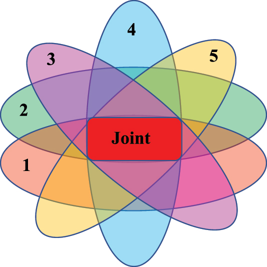
Venn diagram of the joint event. The event Y p1 = n p1, when the probabilities of the responses to property 1 by categories are as in the specific vector p p1, is shown with a semi-transparent brown ellipse 1; similar color ellipses indicate 2 (green) − the event Y p2 = n p2 for property 2; 3 (violet) − the event Y p3 = n p3 for property 3; 4 (blue) − the event Y p4 = n p4 for property 4; and 5 (yellow) − the event Y p5 = n p5 for property 5. The joint (intersection) event, consisting of the corresponding responses to the five properties simultaneously, is highlighted by the central red non-transparent shape. 28
When responses to these five quality properties are independent, the probability of the joint event (joint probability) is the product:
Treating N responses to each quality property as a separate statistical sample, and corresponding frequencies
The product quality index Q index can be formulated as the negative common logarithm (−log10 or − lg) of the estimate of the joint probability:
When the probability estimates
Note that there are no assumptions concerning the contribution of each quality property to the quality index, either being equal or different: the formulated quality index is not a kind of geometric or weighted mean of the property values with probabilities as the weights. Determining the quality characteristics and their categories (the ranges on the ordinal scale), as well as the relevance of these characteristics to consumers, are not the task of this Guide. They are a part of the product specifications in a standard or another regulatory document related to the product.
5.2 The index for responses which might not be independent
When responses to two or more quality properties might not be independent, the probability of the joint (intersection) event P
joint can be represented numerically by a Gaussian copula-based procedure.
101
,
102
This procedure is used for generating samples from a discrete multivariate random variable with the prescribed experimental marginal cumulative distributions
5.3 Variability of the quality index
A representative dataset of responses to each property is necessary for an estimation of the vector of relative frequencies and PMFs by Eq. (1). It may be a dataset containing results of examination of samples from one batch. The quality index characterizes this batch in such a case. When the dataset is accumulated by examination of batches during a specified term, the quality index characterizes the product (and production in the specified term) in general. The variability of the
However, it is important that the
Such quality indices are discussed in Annex A, Example 5, using the described approach for analysis of a dataset related to a sausage from two producers. 28
6 Implementation
In practice, the purposes of comparisons and the number of laboratories (producers) able and ready to participate in a comparison may be different, and the number of test items may be small or large. When a consensus is not achieved (the responses are inhomogeneous), outlying laboratory responses should be investigated. The outlier(s) may be removed from the dataset for calculation if the laboratory finds that the conditions of the experiment were violated. If a violation was not detected, removing outliers is not recommended 1 , 13 , 16 as this action decreases the power of the test and increases the risks of false decisions.
In any case, a fit-for-purpose algorithm is to be elaborated for correct treatment and interpretation of the obtained data, especially in the complex interlaboratory comparisons of responses correlated with chemical composition of an object or correlated responses to different properties of the same product. Such an algorithm can be represented as a flow chart.
6.1 Algorithms for data treatment
When a property of samples of a product of different producers is examined in one laboratory/institution by a group of experienced experts, and the chemical composition of each sample is known from a certificate provided by its producer, a flow chart of data treatment is shown in Fig. 2. It starts from calculation of the frequencies of expert responses (of different categories), and evaluation of the total variation. The next step is decomposition of the total variation into components with the purpose to assess the effects of two factors influencing the variation – “producer” (X1) and “expert” (X2).
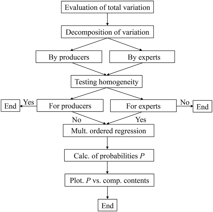
Flow chart of the data treatment for interlaboratory comparison of categorical characteristics of a substance, material, or object. 27
The components of variation obtained are used for testing the hypotheses on homogeneity of the producers (i.e., the responses to their product quality properties) and homogeneity of the experts (their responses to a property of the same product sample). When responses of different experts are inhomogeneous, and/or the responses to different producers are homogeneous, the analysis is ended. Otherwise, it is assumed that the difference between responses to the product quality of different producers is caused by the differences in the product chemical composition. This hypothesis is tested with multinomial ordered logistic regression analysis. If any of the regression coefficients are statistically significant, probabilities of obtaining a response related to a specific category for different components of the chemical composition are calculated. The last step is plotting such probabilities for visualization of the results and their discussion like in Annex A, Example 4.
Another algorithm is necessary, when the chemical composition of each sample of a product under examination is known and correlations between the responses to different properties of the product are considered. Such an algorithm may start from testing the homogeneity of the datasets of chemical composition that able to influence the responses. For samples, for which the hypothesis on homogeneity of the chemical composition is not rejected, ORDANOVA is implemented. Then only testing correlation of the responses to the different quality properties can be performed. If correlation is not statistically significant, a quality index of the product can be calculated by Eq. (25). Otherwise, the quality index is calculated numerically by a Gaussian copula-based procedure as explained in Sec. 5.2 and Annex A, Example 5.
6.2 Limitations
This Guide discusses the risks of false decisions on consensus as probabilities, not considering the severity of their consequences: quality loss, aesthetic and taste worsening in a product, financial loss, etc. There are also typical limitations of the applied methods of mathematical statistics: the use of any model is a simplified reflection of reality; adequacy of the treatment of a dataset of item-to-item (batch-to-batch) and/or expert-to-expert responses; the goodness-of-fit of experimental and theoretical distributions, etc.
Funding source: International Union of Pure and Applied Chemistry
Award Identifier / Grant number: Projects 2021-017-2-500 and 2023-016-1-500
Acknowledgments
The Task Group would like to thank I. Andrić (Croatia), V. N. Naidenko (Russia), M. N. Salikova (Russia) and Y. N. Yariv (Israel) for the help in preparation of the Examples in Annex A of this Guide.
-
Research ethics: Not applicable.
-
Informed consent: Not applicable.
-
Author contributions: All authors have accepted responsibility for the entire content of this manuscript and approved its submission.
-
Use of Large Language Models, AI and Machine Learning Tools: None declared.
-
Conflict of interest: All other authors state no conflict of interest.
-
Research funding: This work was prepared under projects 2021-017-2-500 and 2023-016-1-500 of IUPAC (Funder ID: 10.13039/100006987).
-
Data availability: Not applicable.
Annex A: Examples
Example 1. Calculation of power of the test for nominal variables
A-1-1 Introduction
The aim of this example is to illustrate the dependence of values of power,
A-1-2 Examples of the power calculations for nominal variables
The calculated results for
Power
Power
Note that the axes of the plots in the figures do not start from zero, but correspond to the set ranges (from 3 for
Example 2. A comparison of weld imperfections
A-2-1 Introduction
This example demonstrates the implementation of two-way CATANOVA for a case study of nominal variables in an interlaboratory comparison of responses of technicians who categorized weld imperfections on the images for macroscopic examination. It is also an example of evaluation of the consensus of the comparison participants when their responses are nominal values.
A-2-2 Experiment
Three accredited laboratories participated in the comparison,
25
A-2-3 Implementation of two-way CATANOVA
Numbers of responses by category obtained in each laboratory (technicians 1 and 2) to the 14 imperfections, i.e., frequencies
Numbers of the responses by laboratory, technician, and categories,
| Category, K | Laboratory (X1), i | Total | |||||
|---|---|---|---|---|---|---|---|
| 1 | 2 | 3 | |||||
| Technician (X2), j | |||||||
| 1 | 2 | 1 | 2 | 1 | 2 | ||
| 1 | 1 | 4 | 1 | 4 | 0 | 1 | 11 |
| 2 | 2 | 3 | 3 | 2 | 2 | 2 | 14 |
| 3 | 2 | 2 | 1 | 2 | 1 | 1 | 9 |
| 4 | 6 | 4 | 6 | 2 | 5 | 6 | 29 |
| 5 | 3 | 1 | 3 | 4 | 6 | 4 | 21 |
| Total | 14 | 14 | 14 | 14 | 14 | 14 | 84 |
The individual effect of laboratories as factor
Since
A-2-4 Evaluation of the consensus
Under hypothesis
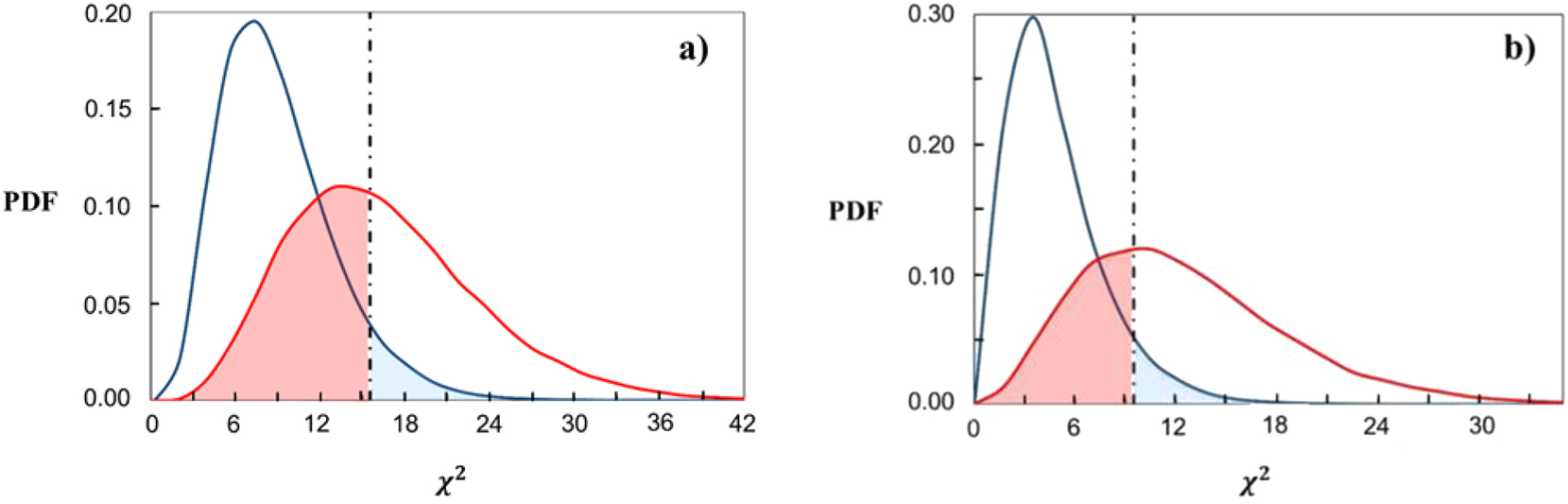
Probability density functions (PDFs) of the chi-square distributions. Plot (a) is for factor
For factor
In other words, a consensus of the laboratories in assessment of the weld imperfections, and an agreement between an experienced technician and a trained novice in a laboratory, were accepted at the level of confidence
Example 3. A comparison of the intensity of odors of drinking water
A-3-1 Introduction
The objective of this example is demonstration of the implementation of two-way ORDANOVA without replication for a case study of ordinal variables in an interlaboratory comparison of sensory responses to the intensity of the odor of drinking water samples, and an evaluation of the consensus of the comparison participants when their responses are ordinal values.
A-3-2 Experiment
Two test items, 1 and 2, were prepared for examination of the intensity of a chlorine and a sulfurous odor, respectively. 26 The components of these items were purchased bottled drinking water (from the same producer and batch), 330 cm3 in a plastic container for each item, and the initial solutions of the pure reagents in glass vials: 3 cm3 of sodium hypochlorite, 0.544 g/dm3, for test item 1 providing a chlorine odor; and 3 cm3 of sodium sulfide, 0.167 g/dm3, for test item 2 providing a sulfurous odor.
The solution of sodium hypochlorite was mixed with the drinking water before use by each participating laboratory to obtain the final concentration of sodium hypochlorite in test item 1 equal to 4.9 mg/dm3. This concentration of sodium hypochlorite corresponds to intensity level 2 of chlorine odor, interpolated between levels 1 and 3 described in the national standard GOST R 57164. 105 The final concentration of sodium sulfide in test item 2 equal to 1.5 mg/dm3 was obtained by mixing its initial solution with the drinking water, also before use by each participating laboratory. This concentration of sodium sulfide corresponds to intensity level 4 of sulfurous odor, interpolated between levels 3 and 5 by ref. 105 .
The assigned categories of the intensity of odor in the prepared items were set according to the preparation procedure. 1 The influence of any lack of chemical homogeneity of the initial solutions on the assigned categories was negligible. The solutions of sodium hypochlorite and sodium sulfide were stable for three weeks, when kept in tightly-closed glassware between temperatures from 4 °C to 20 °C. The stability of the test items 1 and 2 was not relevant, as they were prepared immediately before use.
The components of items 1 and 2 were distributed to the 49 ecological laboratories which participated in the comparison in random order. The examination of the items was performed at a participating laboratory immediately after preparation of the final solutions in the same conditions as for routine water samples, in six categories of the intensity for both the water odors according to the national standard. 105 There are a) imperceptible odor, b) very weak, c) weak – does not cause a disapproving response about the water, d) noticeable – causes a disapproving response, e) distinct – a tester wishes not to drink, and f) very strong – the water is not potable. To each category, the standard assigns the respective numeric score from 0 to 5. The temperature of a test item was measured and adjusted to (20 ± 2) °C by keeping at room temperature. To adjust a test item temperature to (60 ± 5) °C, the flask with the item was immersed in a water bath for heating.
Finally, 45 laboratories reported. Thus, there were factor X1 − laboratory with I = 45 levels; factor X2 − temperature of a water sample with J = 2 levels (j = 1 at 20 °C and j = 2 at 60 °C); K = 6 categories/levels of chlorine or sulfurous odor intensity (k from 0 to 5); n = 1 − one response from each laboratory related to a sample of the specified odor at the specified temperature; N = IJ = 90 responses in total for each chlorine odor and sulfurous odor. 26
A-3-3 Implementation of two-way ORDANOVA without replication
Numbers of the responses (examination results) obtained from all laboratories by categories at the specified temperature of a water sample, i.e., frequencies
Numbers of the responses by a water sample temperature and categories,
| Category, k | Chlorine odor | Total | Sulfurous odor | Total | ||
|---|---|---|---|---|---|---|
| Temperature (X2), j | Temperature (X2), j | |||||
| 1 | 2 | 1 | 2 | |||
| 0 | 2 | 2 | 4 | 0 | 0 | 0 |
| 1 | 24 | 14 | 38 | 0 | 0 | 0 |
| 2 | 10 | 19 | 29 | 0 | 0 | 0 |
| 3 | 9 | 10 | 19 | 10 | 12 | 22 |
| 4 | 0 | 0 | 0 | 17 | 11 | 28 |
| 5 | 0 | 0 | 0 | 18 | 22 | 40 |
| Total | 45 | 45 | 90 | 45 | 45 | 90 |
The total sample variation of the responses for the intensity of chlorine odor is
The significance index of the laboratory factor
A-3-4 Evaluation of the consensus
The proposed algorithm using random MC draws from a multinomial distribution was applied to evaluate the consensus of the laboratories at the given
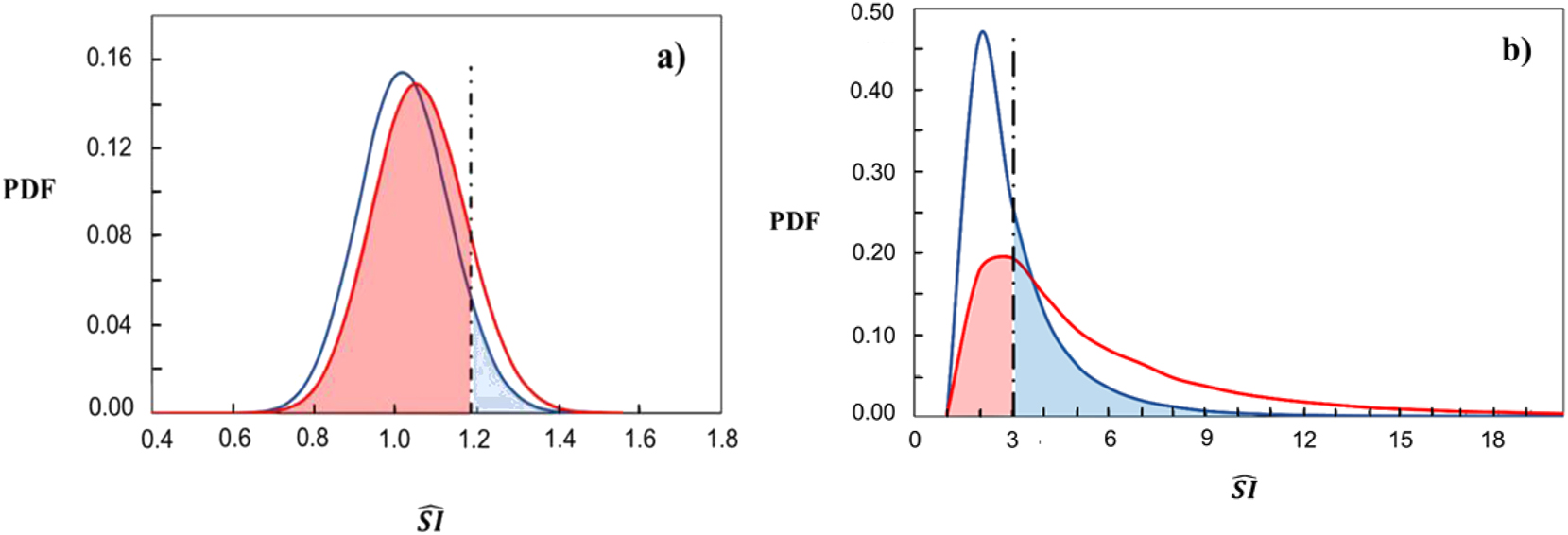
PDFs of the significance index under hypothesis
The blue line shows the PDF of
Note that decreasing the level of confidence (increasing the
Example 4. Multinomial ordered logistic regression of sensory responses to the quality of a sausage from different producers versus the chemical composition of the sausage
A-4-1 Introduction
The objective of the present example is implementation of two-way ORDANOVA without replication in combination with a multinomial ordered logistic regression of sensory responses to the quality of a sausage from different producers, influenced not only by variability of the testing laboratories or their experts, but also by the chemical composition of the object under examination.
A-4-2 Experimental
Samples of boiled-smoked sausage “Moscowskaya” by the national standard GOST R 55455
106
from
A-4-3 Implementation of two-way ORDANOVA without replication
Numbers of responses by experts and categories, i.e., frequencies
Numbers of responses to the quality of sausages by experts and categories,
| Category, k | Appearance | Consistency | Color | Taste | Smell | ||||||||||
|---|---|---|---|---|---|---|---|---|---|---|---|---|---|---|---|
| Experts (X2), j | |||||||||||||||
| 1 | 2 | 3 | 1 | 2 | 3 | 1 | 2 | 3 | 1 | 2 | 3 | 1 | 2 | 3 | |
| 1 | 0 | 0 | 0 | 0 | 0 | 0 | 0 | 0 | 0 | 0 | 0 | 0 | 0 | 0 | 0 |
| 2 | 0 | 0 | 0 | 0 | 0 | 0 | 0 | 0 | 0 | 0 | 0 | 0 | 0 | 0 | 0 |
| 3 | 3 | 0 | 0 | 0 | 0 | 0 | 3 | 1 | 2 | 3 | 3 | 4 | 3 | 2 | 3 |
| 4 | 4 | 3 | 7 | 3 | 3 | 6 | 7 | 4 | 3 | 6 | 4 | 5 | 6 | 5 | 5 |
| 5 | 9 | 13 | 9 | 13 | 13 | 10 | 6 | 11 | 11 | 7 | 9 | 7 | 7 | 9 | 8 |
| Total | 16 | 16 | 16 | 16 | 16 | 16 | 16 | 16 | 16 | 16 | 16 | 16 | 16 | 16 | 16 |
Total variation
Results of two-way ORDANOVA in the study of the “Moscowskaya” sausage by different producers.
| Property |
|
|
|
|
|
|
|
|
|---|---|---|---|---|---|---|---|---|
| Appearance | 0.287 | 0.184 | 0.103 | Producer | 0.162 | 1.769 | 15 | 1.432 |
| Expert | 0.022 | 1.801 | 2 | 2.686 | ||||
| Consistency | 0.187 | 0.112 | 0.075 | Producer | 0.104 | 1.740 | 15 | 1.550 |
| Expert | 0.008 | 0.980 | 2 | 2.892 | ||||
| Color | 0.352 | 0.251 | 0.101 | Producer | 0.227 | 2.019 | 15 | 1.422 |
| Expert | 0.024 | 1.621 | 2 | 2.554 | ||||
| Taste | 0.414 | 0.293 | 0.121 | Producer | 0.289 | 2.186 | 15 | 1.403 |
| Expert | 0.004 | 0.246 | 2 | 2.521 | ||||
| Smell | 0.389 | 0.295 | 0.094 | Producer | 0.292 | 2.351 | 15 | 1.408 |
| Expert | 0.004 | 0.210 | 2 | 2.510 |
There is a statistically significant difference at 95 % level of confidence between the producers related to all the quality parameters of the sausage (appearance, consistency, color, taste, and smell). This difference is called the “inhomogeneity” of the producers. At the same time, the significance index values of the expert factor do not exceed its critical value at 95 % level of confidence, i.e., the null hypotheses H 0 on the “homogeneity” of expert responses regarding to each of the five sausage properties were not rejected.
A-4-4 Implementation of the multinomial ordered logistic regression
The multinomial ordered logistic regression model by Eq. (20) was fitted to the component contents in order to predict appearance, color, taste, and smell, assessed by experts according to the three categories shown in Table 4, k = 3, 4, and 5. A logistic regression for dichotomous (binary) outcome variables was used for prediction of consistency, since the corresponding expert responses in Table 4 were only of two categories, k = 4 and 5. Since for each categorical variable, the responses were found to be homogeneous among the three experts at the ORDANOVA study, all their outcomes were taken together, constituting the set of values to be used in the regression. Intervals of the sausage main component contents in the certificates of the producers, taken into account in the regression, as well as the means and standard deviations of the contents (mass fraction expressed in %) are shown in Table 6. The calculation results are presented in Table 7, where the estimates for γ k0 and η i coefficients are reported with their standard errors and 95 % confidence intervals (from 2.5 % to 97.5 % quantile). The estimated odds ratios, derived by exponentiating the coefficients, and the McFadden’s pseudo-R 2 values by Eq. (22) are also shown in Table 7. 27
Statistics of the chemical composition of samples of the “Moscowskaya” sausage.
| Statistics | Protein, c 1, % | Fat, c 2, % | Moisture, c 3, % | Salt, c 4, % |
|---|---|---|---|---|
| Minimum | 13.7 | 19.9 | 53.5 | 2.2 |
| Maximum | 19.5 | 26.4 | 59.5 | 3.5 |
| Mean | 15.8 | 23.0 | 56.0 | 2.6 |
| Standard deviation | 1.4 | 4.6 | 1.9 | 0.3 |
Results of the multinomial ordered logistic regression analysis.
| Property | Coefficient | Value | Standard error | 2.5 % | 97.5 % | Odds ratio | Pseudo-R 2 |
|---|---|---|---|---|---|---|---|
| γ k0 (3|4) | 108.31 | 0.01 | 108.30 | 108.32 | 1.09 × 1047 | ||
| γ k0 (4|5) | 110.71 | 0.61 | 109.51 | 111.91 | 1.21 × 1048 | ||
| Appearance | η 1 | 1.65 | 0.30 | 1.06 | 2.24 | 5.20 | |
| η 2 | 0.95 | 0.10 | 0.76 | 1.14 | 2.58 | 0.13 | |
| η 3 | 1.24 | 0.07 | 1.10 | 1.38 | 3.44 | ||
| η 4 | −2.22 | 1.31 | −4.78 | 0.34 | 0.11 | ||
| γ k0 | −113.55 | 66.07 | −243.05 | 15.95 | 4.85 × 10−50 | ||
| Consistency | η 1 | 1.35 | 0.69 | 0.00 | 2.71 | 3.87 | 0.11 |
| η 2 | 1.08 | 0.56 | −0.01 | 2.18 | 2.95 | ||
| η 3 | 1.22 | 0.78 | −0.30 | 2.74 | 3.40 | ||
| γ k0 (3|4) | 21.76 | 0.01 | 21.75 | 21.78 | 2.83 × 10⁹ | ||
| γ k0 (4|5) | 23.56 | 0.44 | 22.69 | 24.42 | 1.70 × 10¹⁰ | ||
| Color | η 1 | 0.56 | 0.25 | 0.07 | 1.05 | 1.75 | |
| η 2 | −0.03 | 0.10 | −0.23 | 0.17 | 0.97 | 0.09 | |
| η 3 | 0.31 | 0.06 | 0.18 | 0.43 | 1.36 | ||
| η 4 | −0.51 | 1.28 | −3.02 | 1.99 | 0.60 | ||
| Color* | γ k0 (3|4) | 26.80 | 11.85 | 3.57 | 50.02 | 4.34 × 10¹¹ | 0.09 |
| γ k0 (4|5) | 28.59 | 11.93 | 5.21 | 51.97 | 2.60 × 10¹² | ||
| η 1 | 0.56 | 0.27 | 0.07 | 1.05 | 1.75 | ||
| η 3 | 0.36 | 0.18 | 0.18 | 0.43 | 1.43 | ||
| Taste | γ k0 (3|4) | 202.04 | 0.00 | 202.03 | 202.04 | 5.55 × 1087 | |
| γ k0 (4|5) | 204.47 | 0.55 | 203.39 | 205.55 | 6.31 × 1088 | ||
| η 1 | 2.87 | 0.30 | 2.28 | 3.46 | 17.61 | 0.28 | |
| η 2 | 1.73 | 0.09 | 1.54 | 1.91 | 5.62 | ||
| η 3 | 2.33 | 0.07 | 2.19 | 2.47 | 10.27 | ||
| η 4 | −4.42 | 1.51 | −7.37 | −1.47 | 0.01 | ||
| γ k0 (3|4) | 218.42 | 0.00 | 218.41 | 218.42 | 7.19 × 1094 | ||
| Smell | γ k0 (4|5) | 221.26 | 0.62 | 220.04 | 222.47 | 1.23 × 1096 | |
| η 1 | 3.25 | 0.35 | 2.58 | 3.93 | 25.92 | ||
| η 2 | 1.99 | 0.10 | 1.80 | 2.18 | 7.33 | 0.32 | |
| η 3 | 2.41 | 0.08 | 2.26 | 2.57 | 11.18 | ||
| η 4 | −4.42 | 1.54 | −7.43 | −1.40 | 0.01 |
-
*A shorted model of probability of the color category versus contents of protein and moisture.
For example, the model by Eq. (20) of category k=3 for appearance is logit
The corresponding odds ratio
Note, if a confidence interval does not cross zero, the parameter estimate is statistically significant. However, the confidence interval for the estimate η 4 = 2.22 (of the regression coefficient of the salt content c 4) crosses zero and this means that η 4 is statistically not significant here. In other words, the salt content values in the interval shown in Table 6 do not influence the probability of appearance category of a whole sausage.
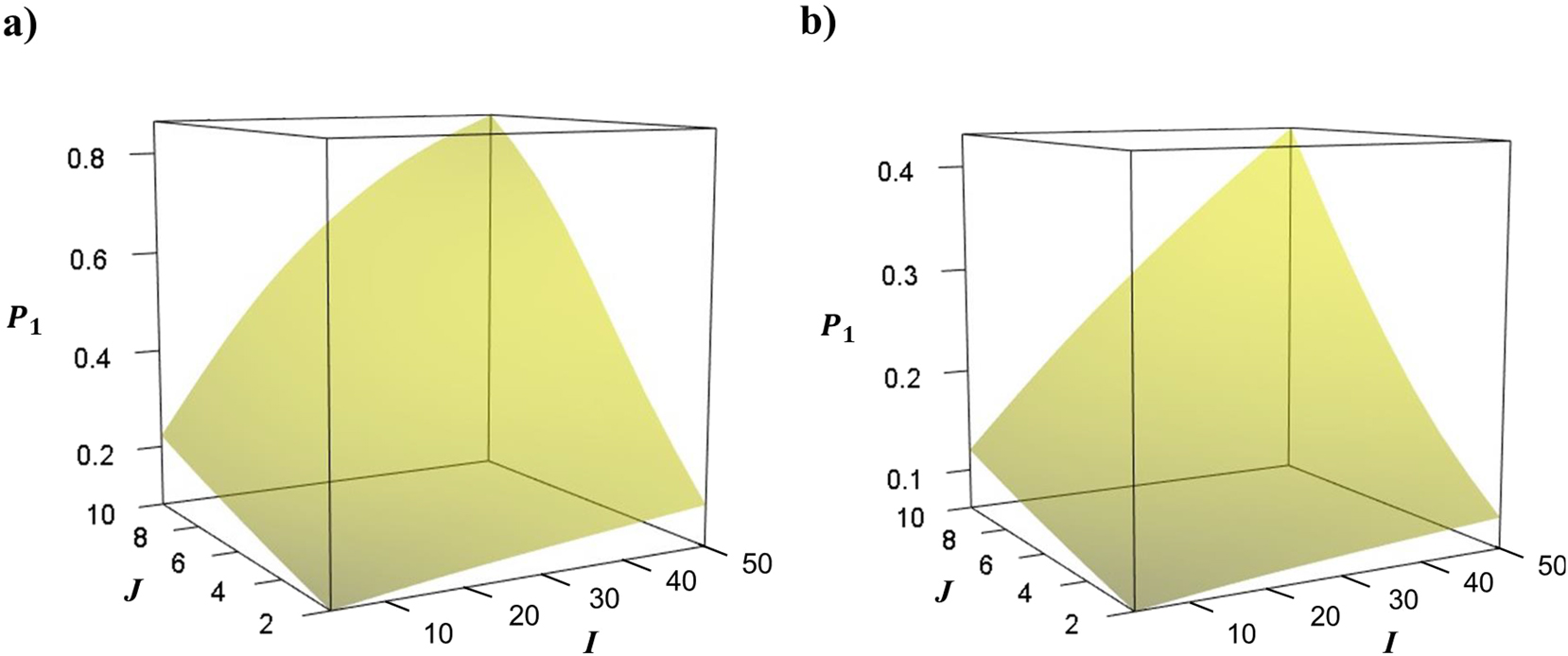
Probabilities P of obtaining a response of category k by dependence on protein content c
1, calculated at the mean values of contents of other main components (Table 6), are shown on Fig. 7a. In the case of three categories of the observed responses (k = 3, 4, and 5), the probability
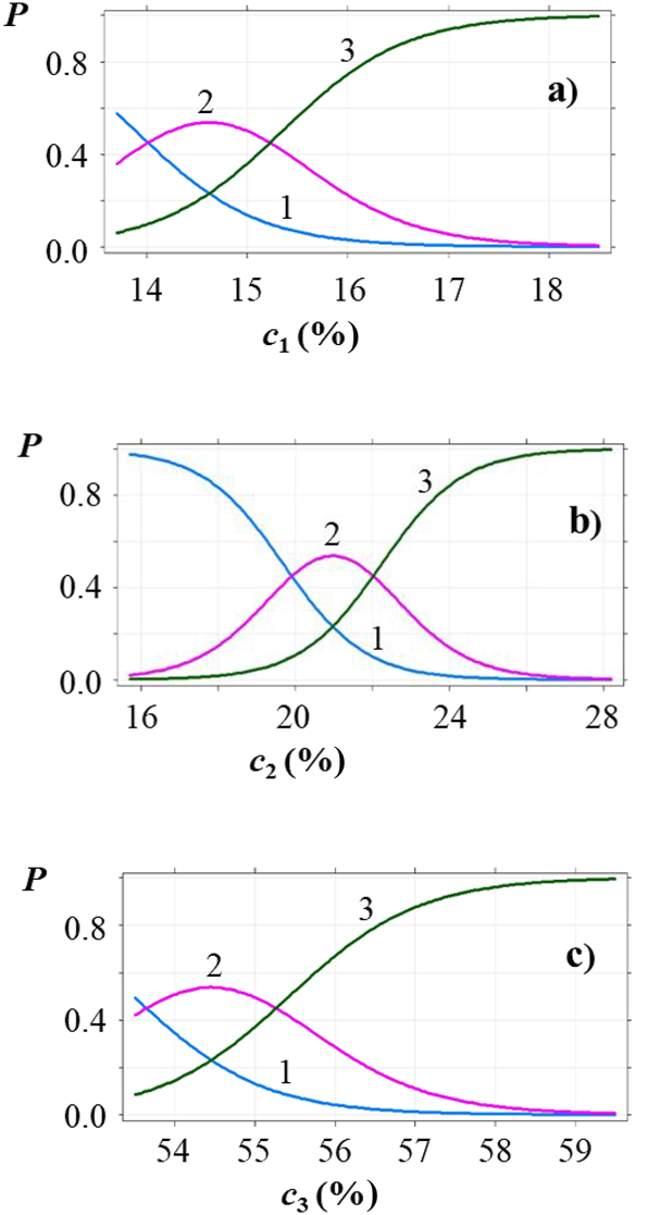
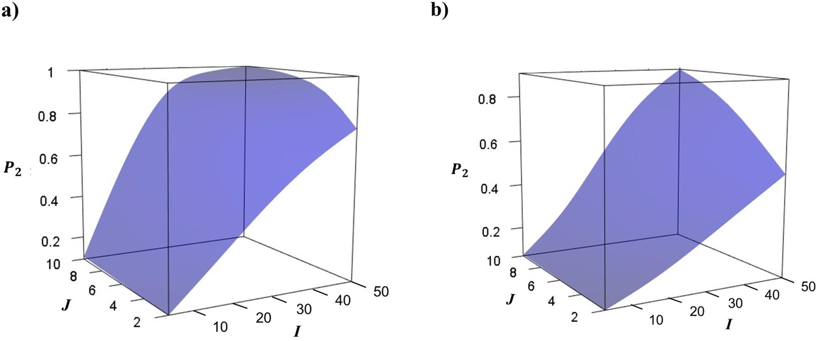
Probabilities P of responses of different appearance categories in dependence on content of (a) protein c 1, (b) fat c 2, and (c) moisture c 3, mass fractions expressed in %. Each plot is calculated at contents of other main components equal to their observed mean values (Table 6). Line 1 is for category “satisfactory” (k = 3), line 2 for category “good” (k = 4), and line 3 for category “excellent” (k = 5). 27
The full models for taste and smell are the best fitting models among the qualitative sausage properties: their McFadden’s pseudo-R 2 values in Table 7 are about two to three times greater than those for appearance, color, and consistency. In general, the maximum probability of responses of each category of taste and smell is reached at increasing contents of the influencing main components. Similar effects are also observed in the plots in Fig. 7 for appearance: the first category reaching its maximum probability in the studied ranges of the component contents is 3, then 4, and finally 5, i.e., higher categories are more probable with greater contents of components. However, the salt contents in the interval considered in this study do not significantly influence responses on appearance, color, and consistency. At the same time, taste and smell are influenced by the salt contents in a reverse order than contents of other main components: the greater the salt content, the lower category is the more probable.
The probabilities of responses of the excellent quality category
Example 5. Comparison of the multisensory quality index values of a sausage of two producers
A-5-1 Introduction
This example demonstrates implementation of two-way ORDANOVA without replication for calculation of the multisensory multinomial quality index of a product, considering possible correlation of the responses to the different quality properties of the same product. It is shown how the index could be used for comparison of quality of this product from two producers.
A-5-2 Experiment
The dataset used here included results of sensory analysis and chemical analysis of the same boiled-smoked sausage “Moscowskaya” 106 as in Example 4. However, this time, the data were accumulated from each of two manufacturers during two years of the production. There were I 1 = 26 batches i = 1, 2, …, 26 of the first sausage manufacturer, named hereafter “producer 1”, and I 2 = 54 batches i = 1, 2, …, 54 of the second manufacturer, named “producer 2”. Five quality sensory properties of the sausage in a batch were examined without replication at each producer factory by its J = 5 experienced experts j = 1, 2, …, 5: a) appearance and packaging, named “appearance”; b) consistency; c) color and appearance of cut sausage, named “color”; d) taste; and f) smell. An expert response related to each quality property was ordered by K = 5 categories k from “very bad” to “excellent”, k = 1, 2, …, 5. A total N 1 = I 1 × J = 130 responses were obtained for each property, and hence 130 × 5 = 650 responses to the five properties of the sausage of producer 1, while for the sausage of producer 2, there were N 2 = I 2 × J = 270 responses to each property and 270 × 5 = 1,350 responses to the five properties. Contents (measured mass fractions expressed in %) of the m = 4 main components were taken from the batch certificates of the producer, included I 1 × m = 104 quantitative values of producer 1 and I 2 × m = 216 such values of producer 2, characterizing the sausage chemical compositions. 28
A-5-3 Statistics of the chemical composition
The intervals of mass fractions of the main sausage components expressed in % (protein c 1, fat c 2, moisture c 3, and salt c 4), minimum and maximum measured values, as well as the mean and standard deviations of the mass fractions of I 1 = 26 batches of producer 1 and I 2 = 54 batches of producer 2, are presented in Table 8.
Statistics of the chemical composition of the sausage from each of two producers.
| Producer | Statistic | Protein, c 1, % | Fat, c 2, % | Moisture, c 3, % | Salt, c 4, % |
|---|---|---|---|---|---|
| 1 | Minimum | 13.71 | 27.14 | 50.11 | 1.85 |
| Maximum | 15.60 | 31.02 | 56.74 | 2.47 | |
| Mean | 14.85 | 29.35 | 53.92 | 2.21 | |
| Standard deviation | 0.53 | 0.93 | 1.53 | 0.13 | |
| 2 | Minimum | 16.34 | 20.69 | 48.45 | 1.50 |
| Maximum | 20.40 | 31.24 | 57.98 | 2.80 | |
| Mean | 17.89 | 25.10 | 53.81 | 2.38 | |
| Standard deviation | 0.74 | 2.33 | 2.24 | 0.26 |
Homogeneity of the two standard deviations (the null hypothesis of equality of variances) was tested using a two-sided Fisher’s test at 95 % level of confidence and degrees of freedom for the numerator I 1 − 1 = 25, and I 2 − 1 = 53 for the denominator. The null hypothesis is rejected for fat, moisture, and salt, and not rejected for protein. Thus, chemical compositions of the sausages of the two producers were, in general, different. Because chemical composition may influence expert responses to the sausage quality properties as shown in Example 4, the ordinal data subsets of producer 1 and producer 2 were treated separately.
A-5-4 Implementation of two-way ORDANOVA without replication
Numbers of the responses (frequencies n jk ) are shown in Table 9 for each quality property of the sausage. The high categories of the quality properties of the product are to be expected: otherwise, a consumer would not buy the sausage in a store.
Numbers of the responses by experts and categories n jk from each of two producers.
| Property | Expert, j | Producer 1, category k | Producer 2, category k | ||||||||
|---|---|---|---|---|---|---|---|---|---|---|---|
| 1 | 2 | 3 | 4 | 5 | 1 | 2 | 3 | 4 | 5 | ||
| Appearance | 1 | 0 | 0 | 0 | 4 | 22 | 0 | 0 | 0 | 0 | 54 |
| 2 | 0 | 0 | 0 | 3 | 23 | 0 | 0 | 0 | 5 | 49 | |
| 3 | 0 | 0 | 0 | 2 | 24 | 0 | 0 | 0 | 0 | 54 | |
| 4 | 0 | 0 | 0 | 0 | 26 | 0 | 0 | 0 | 3 | 51 | |
| 5 | 0 | 0 | 0 | 0 | 26 | 0 | 0 | 0 | 1 | 53 | |
| Consistency | 1 | 0 | 0 | 1 | 12 | 13 | 0 | 0 | 0 | 2 | 52 |
| 2 | 0 | 0 | 1 | 8 | 17 | 0 | 0 | 0 | 7 | 47 | |
| 3 | 0 | 0 | 0 | 10 | 16 | 0 | 0 | 0 | 1 | 53 | |
| 4 | 0 | 0 | 0 | 7 | 19 | 0 | 0 | 0 | 3 | 51 | |
| 5 | 0 | 0 | 0 | 10 | 16 | 0 | 0 | 0 | 2 | 52 | |
| Color | 1 | 0 | 0 | 0 | 19 | 7 | 0 | 0 | 0 | 3 | 51 |
| 2 | 0 | 0 | 0 | 10 | 16 | 0 | 0 | 0 | 9 | 45 | |
| 3 | 0 | 0 | 0 | 13 | 13 | 0 | 0 | 0 | 4 | 50 | |
| 4 | 0 | 0 | 0 | 9 | 17 | 0 | 0 | 0 | 3 | 51 | |
| 5 | 0 | 0 | 2 | 11 | 13 | 0 | 0 | 0 | 5 | 49 | |
| Taste | 1 | 0 | 0 | 1 | 11 | 14 | 0 | 0 | 0 | 4 | 50 |
| 2 | 0 | 0 | 1 | 8 | 17 | 0 | 0 | 0 | 8 | 46 | |
| 3 | 0 | 0 | 0 | 8 | 18 | 0 | 0 | 0 | 4 | 50 | |
| 4 | 0 | 0 | 1 | 5 | 20 | 0 | 0 | 0 | 7 | 47 | |
| 5 | 0 | 0 | 0 | 6 | 20 | 0 | 0 | 0 | 7 | 47 | |
| Smell | 1 | 0 | 0 | 0 | 3 | 23 | 0 | 0 | 0 | 2 | 52 |
| 2 | 0 | 0 | 0 | 2 | 24 | 0 | 0 | 0 | 7 | 47 | |
| 3 | 0 | 0 | 0 | 3 | 23 | 0 | 0 | 0 | 2 | 52 | |
| 4 | 0 | 0 | 0 | 1 | 25 | 0 | 0 | 0 | 3 | 51 | |
| 5 | 0 | 0 | 0 | 3 | 23 | 0 | 0 | 0 | 5 | 49 | |
Total variation
Results of two-way ORDANOVA of the responses to the quality characteristics of the sausage from each of two producers during two years of its production.
| Property |
|
|
|
X1 & X2 |
|
|
|
|
|---|---|---|---|---|---|---|---|---|
| Producer 1 | ||||||||
|
|
||||||||
| Appearance | 0.064 | 0.031 | 0.033 | Batch | 0.027 | 2.203 | 25 | 1.464 |
| Expert | 0.004 | 1.895 | 4 | 2.192 | ||||
| Consistency | 0.250 | 0.121 | 0.129 | Batch | 0.115 | 2.366 | 25 | 1.416 |
| Expert | 0.006 | 0.763 | 4 | 2.268 | ||||
| Color | 0.265 | 0.152 | 0.113 | Batch | 0.133 | 2.585 | 25 | 1.429 |
| Expert | 0.019 | 2.304 | 4 | 2.290 | ||||
| Taste | 0.238 | 0.123 | 0.115 | Batch | 0.115 | 2.497 | 25 | 1.406 |
| Expert | 0.008 | 1.040 | 4 | 2.189 | ||||
| Smell | 0.084 | 0.039 | 0.045 | Batch | 0.038 | 2.318 | 25 | 1.455 |
| Expert | 0.001 | 0.364 | 4 | 2.316 | ||||
|
|
||||||||
| Producer 2 | ||||||||
|
|
||||||||
| Appearance | 0.032 | 0.013 | 0.019 | Batch | 0.012 | 1.809 | 53 | 1.342 |
| Expert | 0.001 | 2.691 | 4 | 2.293 | ||||
| Consistency | 0.053 | 0.020 | 0.033 | Batch | 0.018 | 1.779 | 53 | 1.312 |
| Expert | 0.002 | 1.934 | 4 | 2.283 | ||||
| Color | 0.081 | 0.038 | 0.043 | Batch | 0.036 | 2.290 | 53 | 1.302 |
| Expert | 0.002 | 1.412 | 4 | 2.293 | ||||
| Taste | 0.099 | 0.069 | 0.030 | Batch | 0.068 | 3.477 | 53 | 1.303 |
| Expert | 0.001 | 0.654 | 4 | 2.321 | ||||
| Smell | 0.065 | 0.046 | 0.019 | Batch | 0.045 | 3.466 | 53 | 1.312 |
| Expert | 0.001 | 1.326 | 4 | 2.287 | ||||
There are significant differences between the studied batches of producer 1 as
However, there is no statistically significant difference at 95 % level of confidence between the experts’ responses related to appearance, consistency, taste, and smell. The
The values of the significance index
The homogeneity of the responses of the five experts of each producer allows the use of the subset of each producer’s data for calculation of its sausage multinomial multisensory quality index.
A-5-5 Testing correlation of the responses to the different quality properties
Spearman’s rho correlation coefficient, calculated with the IBM SPSS software, 108 is used here as a nonparametric measure of the strength and direction of association that exists between responses to two quality properties as ordinal variables. The association is complete (the variables are strongly correlated), when the coefficient value achieves ±1, and the association is absent when the coefficient value is zero. The matrices of Spearman’s rho correlation coefficients for N 1 = 130 pairs of responses to quality properties of the sausage of producer 1 (for each pair of the five properties), and similar for N 2 = 270 pairs related to the sausage of producer 2, are presented in Table 11.
Spearman’s rho correlation coefficients for expert evaluation of quality properties of sausages from producer 1 and producer 2.
| Properties | Appearance | Consistency | Color | Taste | Smell |
|---|---|---|---|---|---|
| Producer 1 | |||||
|
|
|||||
| Appearance | 1.000 | −0.027 | 0.207 | −0.121 | 0.018 |
| Consistency | −0.027 | 1.000 | 0.118 | 0.088 | 0.022 |
| Color | 0.207 | 0.118 | 1.000 | 0.037 | 0.052 |
| Taste | −0.121 | 0.088 | 0.037 | 1.000 | −0.049 |
| Smell | 0.018 | 0.022 | 0.052 | −0.049 | 1.000 |
|
|
|||||
| Producer 2 | |||||
|
|
|||||
| Appearance | 1.000 | 0.585 | 0.522 | 0.394 | 0.514 |
| Consistency | 0.585 | 1.000 | 0.549 | 0.480 | 0.439 |
| Color | 0.522 | 0.549 | 1.000 | 0.387 | 0.372 |
| Taste | 0.394 | 0.480 | 0.387 | 1.000 | 0.778 |
| Smell | 0.514 | 0.439 | 0.372 | 0.778 | 1.000 |
The SPSS software output contains also the two-tailed significance probability of making the wrong decision on correlation of the ordinal variables when the null hypothesis on their uncorrelation is true (the probability α of a Type I error). From these calculations for producer 1, the null hypothesis was not rejected at 95 % level of confidence (α = 5 %) and correlation was not supported for responses to all the quality properties apart of the pair “appearance-color”. For this pair, the null hypothesis was not rejected at 99 % level of confidence (α = 1 %). For producer 2, the calculated correlation coefficients in Table 11 are considerably larger than for producer 1. The negligible probability of a Type 1 error here (α = 0 %) for any pair of tested quality properties indicating a high degree of correlation.
The reasons for the different correlation matrices of responses to the properties of the same sausage of two producers were not studied in this work. However, they are responses of two different groups of experts, each group employed by one producer for the sensory examination of its product.
Note that independent variables are necessarily uncorrelated. Therefore, the multinomial multisensory quality index was calculated for the sausage of producer 1 as a case study of independent responses to the quality properties, while the index for the sausage of producer 2 was evaluated considering that the responses to its quality properties were correlated.
A-5-6 Calculation of the quality index for independent responses
Table 12 gives the vector of frequencies by categories
Statistics for calculation of the quality index
| Statistic | Category, k | Appearance | Consistency | Color | Taste | Smell |
|---|---|---|---|---|---|---|
|
|
1 | 0 | 0 | 0 | 0 | 0 |
| 2 | 0 | 0 | 0 | 0 | 0 | |
| 3 | 0 | 2 | 2 | 3 | 0 | |
| 4 | 9 | 47 | 62 | 38 | 12 | |
| 5 | 121 | 81 | 66 | 89 | 118 | |
|
|
1 | 0 | 0 | 0 | 0 | 0 |
| 2 | 0 | 0 | 0 | 0 | 0 | |
| 3 | 0 | 0.0154 | 0.0154 | 0.0231 | 0 | |
| 4 | 0.0692 | 0.3615 | 0.4769 | 0.2923 | 0.0923 | |
| 5 | 0.9308 | 0.6231 | 0.5077 | 0.6846 | 0.9077 | |
|
|
0.1366 | 0.0199 | 0.0192 | 0.0175 | 0.1200 |
When the joint probability is considered that the ideal sausage (having category “excellent” for each property) will be produced, then
A-5-7 Calculation of the quality index for correlated responses
The GenOrd package implementing a Gaussian copula-based procedure
109
was applied for simulation of the discrete multivariate random variables with the given correlation matrix and marginal distributions. A large number (106) of samples of N
2 = 270 occurrences of the multivariate quantities (expert responses to appearance, consistency, color, taste, and smell) were simulated by R function “ordsample”, taking into account the experimental marginal distributions for appearance
The numerical estimate of the joint probability
Note that the minor correlation detected in the dataset of producer 1 (Table 11) for the pair “appearance-color” was assumed negligible for simplicity. To check if this assumption was sustainable, the original (experimental) correlation matrix was also applied. The corresponding quality index value was
In general, the multinomial multisensory quality index value of producer 2 is less than that of producer 1 by about two units, i.e., the probability of the joint event differs by about two orders of magnitude. Therefore, the quality of the sausage manufactured by producer 2 is considered better in the sense that deviations of this sausage quality properties from the claimed ones are less probable.
When the joint probability is considered that the ideal sausage having a category “excellent” for each property will be produced, the quality index
Membership of sponsoring bodies
The present membership of the IUPAC Analytical Chemistry Division (V) is
President: D. Craston (UK); Past President: D. Shaw (USA); Secretary: L. Torsi (Italy); Titular Members: J. Barek (Czech), R. Burks (USA), F. Emmerling (Germany), H. Li (China), V. Peterson (Australia), S. Ražić (Serbia), A. Tintaru (France); Associate Members: E.M.M. Flores (Brazil), I. Leito (Estonia), F. Pitcitelli (Italy), T. Pradeep (India), M. Ramalingam (Malaysia), T. Takeuchi (Japan); National Representatives: R. Apak (Turkey), V. Baranovskaya (Russia), P. Forbes (South Africa), Gábor Galbács (Hungary), N. Galic (Croatia), P. Jarujamrus (Thailand), I. Kuselman (Israel), M. Piston (Uruguay), D. van Oevelen (Netherlands), S.K. Wiedmer (Finland); Emeritus Fellows: D.B. Hibbert (Australia), J. Labuda (Slovakia), M.C.F. Magalhães (Portugal).
The present membership of the IUPAC Subcommittee on Metrology in Chemistry is
Chair: D.B. Hibbert (Australia); Members : E.M.M. Flores (Brazil), J. Meija (Canada), Z. Mester (Canada), H. Li (China), I. Leito (Estonia), S.K. Wiedmer (Finland), S.K. Aggrawal (India), F.R. Pennecchi (Italy), I. Kuselman (Israel), M. Ramalingam (Malaysia), M.F. Camões (Portugal), R.J.N.B. da Silva (Portugal), V. Baranovskaya (Russia), A. Botha (South Africa), D. Craston (UK), S.L.R. Ellison (UK), D. Shaw (USA).
The present membership of the Cooperation of International Traceability in Analytical Chemistry (CITAC) is
Chair: Z. Mester (Canada); Past Chair: B. Guetler (Germany); Vice - Chair: R.J.N.B. da Silva (Portugal); Secretary: F.R. Lourenço (Brazil); Members: A. Squirrell (Australia), M. Horsky (Austria), W. Wegscheider, deceased (Austria), O. P. de Oliveira Junior (Brazil), V. Ponçano (Brazil), T.R.L. Dadamos (Brazil), J.E.S. Sarkis (Brazil), H. Li (China), T. Näykki (Finland), P. Fisicaro (France), S.G. Walch (Germany), I. Papadakis (Greece), D.W.M. Sin (Hong Kong, P. R. China), P. K. Gupta (India), M. Nabi (Iran), M. Walsh (Ireland), I. Kuselman (Israel), F.R. Pennecchi (Italy), M. Sega (Italy), T. Fujimoto (Japan), R.B. Khousam (Lebanon), O. Zakaria (Malaysia), Y.M. Nakanishi (Mexico), L. Samuel (New Zealand), V. Baranovskaya (Russia), N. Oganyan (Russia), T.L. Teo (Singapore), A. Botha (South Africa), M. Obkircher (Switzerland), S. Wunderli (Switzerland), R. Kaarls (the Netherlands), R.J.C. Brown (UK), S.L.R. Ellison (UK), V. Iyengar (USA), J. D. Messman (USA).
The membership of the Task Group is
Chair: I. Kuselman (Israel); Members : P.S. Cheow (Singapore, project 2021-017-2-500), A. Botha (South Africa, project 2023-016-1-500), T. Gadrich (Israel), D. B. Hibbert (Australia), F.R. Pennecchi (Italy), A.A. Semenova (Russia).
References
1. ISO/IEC 17043:2023. Conformity Assessment – General Requirements for the Competence of Proficiency Testing Providers; International Organization for Standardization: Geneva, 2023.Search in Google Scholar
2. ISO 17034:2016. General Requirements for the Competence of Reference Material Producers; International Organization for Standardization: Geneva, 2016.Search in Google Scholar
3. ISO 5725-1:2023. Accuracy (Trueness and Precision) of Measurement Methods and Results — Part 1: General Principles and Definitions; The International Organization for Standardization: Geneva, 2023.Search in Google Scholar
4. Magnusson, B.; Örnemark, U., Eds. In The Fitness for Purpose of Analytical Methods – A Laboratory Guide to Method Validation and Related Topics, EURACHEM Guide, 2nd ed., 2014. Available from: http://www.eurachem.org.Search in Google Scholar
5. International Bureau of Weights and Measures (BIPM). The BIPM Key Comparison Database (KCDB): Sèvres, France, 2024. Available from: https://www.bipm.org/kcdb/.Search in Google Scholar
6. Consultative Committee for Amount of Substance: Metrology in Chemistry and Biology (CCQM). Estimation of a Consensus KCRV and Associated Degrees of Equivalence. CCQM Guidance note; International Bureau of Weights and Measures (BIPM): Sèvres, France, 2013. Available from: https://www.bipm.org/documents/20126/28430045/working-document-ID-5794/49d366bc-295f-18ca-c4d3-d68aa54077b5.Search in Google Scholar
7. Ellison, S. L. R. Consistency Plots: A Simple Graphical Tool for Investigating Agreement in Key Comparisons. Accredit. Qual. Assur. 2022, 27, 341–348. https://doi.org/10.1007/s00769-022-01520-z.Search in Google Scholar
8. Koepke, A.; Lafarge, T.; Possolo, A.; Toman, B. Consensus Building for Interlaboratory Studies, Key Comparisons, and Meta-analysis. Metrologia 2017, 54, S34–S62. https://doi.org/10.1088/1681-7575/aa6c0e.Search in Google Scholar
9. Possolo, A. Interlaboratory Consensus Building Challenge. Anal. Bioanal. Chem. 2020, 412, 3955–3956. https://doi.org/10.1007/s00216-020-02695-5.Search in Google Scholar PubMed
10. Possolo, A. Solution to Interlaboratory Consensus Building Challenge. Anal. Bioanal. Chem. 2021, 413, 3–5. https://doi.org/10.1007/s00216-020-03053-1.Search in Google Scholar PubMed
11. Tutmez, B. Relative Uncertainty-based Bayesian Interlaboratory Consensus Building. Sci. Total Environ. 2023, 870, 161977. https://doi.org/10.1016/j.scitotenv.2023.161977.Search in Google Scholar PubMed
12. Bodnar, O.; Bodnar, T. Bayesian Estimation in Multivariate Inter-laboratory Studies with Unknown Covariance Matrices. Metrologia 2023, 60, 054003. https://doi.org/10.1088/1681-7575/acee03.Search in Google Scholar
13. ISO 13528:2022. Statistical Methods for Use in Proficiency Testing by Interlaboratory Comparison; International Organization for Standardization: Geneva, 2022.Search in Google Scholar
14. Thompson, M.; Ellison, S. L. R. Dark Uncertainty. Accredit. Qual. Assur. 2011, 16, 483–487. https://doi.org/10.1007/s00769-011-0803-0.Search in Google Scholar
15. Thompson, M. A Properly Developed Consensus from a Proficiency Test is, for All Practical Purposes, Interchangeable with a Certified Value for a Matrix Reference Material Derived from an Interlaboratory Comparison. Geostand. Geoanalytical. Res. 2017, 42, 12195–96. https://doi.org/10.1111/ggr.12195.Search in Google Scholar
16. ISO Guide 33405:2024. Reference Materials − Approaches for Characterization and Assessment of Homogeneity and Stability; International Organization for Standardization: Geneva, 2024.Search in Google Scholar
17. ISO 5725-2:2019. Accuracy (Trueness and Precision) of Measurement Methods and Results — Part 2: Basic Method for the Determination of Repeatability and Reproducibility of a Standard Measurement Method; International Organization for Standardization: Geneva, 2019.Search in Google Scholar
18. Merkatas, C.; Toman, B.; Possolo, A.; Schlamminger, S. Shades of Dark Uncertainty and Consensus Value for the Newtonian Constant of Gravitation. Metrologia 2019, 56, 054001. https://doi.org/10.1088/1681-7575/ab3365.Search in Google Scholar
19. Hodges, J. T.; Viallon, J.; Brewer, P. J.; Drouin, B. J.; Gorshelev, V.; Janssen, C.; Lee, S.; Possolo, A.; Smith, M. A. H.; Walden, J.; Wielgosz, R. I. Recommendation of a Consensus Value of the Ozone Absorption Cross-section at 253.65 nm Based on a Literature Review. Metrologia 2019, 56, 034001. https://doi.org/10.1088/1681-7575/ab0bdd.Search in Google Scholar
20. Jackson, D.; Bowden, J.; Baker, R. How Does the DerSimonian and Laird Procedure for Random Effects Meta-analysis Compare with its More Efficient But Harder to Compute Counterparts? J. Stat. Plan. Inference 2010, 140, 961–970. https://doi.org/10.1016/j.jspi.2009.09.017.Search in Google Scholar
21. Hoffman, J. I. E. In Basic Biostatistics for Medical and Biomedical Practitioners; Academic Press, 2019, 2nd ed.; pp. 621–629. Chapter 36 − Meta-Analysis.10.1016/B978-0-12-817084-7.00036-XSearch in Google Scholar
22. Agresti, A. Categorical Data Analysis, 3rd ed.; John Wiley & Sons: Hoboken, NJ, 2013.Search in Google Scholar
23. JCGM 200:2012. International Vocabulary of Metrology — Basic and General Concepts and Associated Terms (VIM), 3rd ed.; Join Committee for Guides in Metrology (JCGM), International Bureau of Weights and Measures (BIPM): Sèvres, France, 2012. Available from: http://www.bipm.org/en/publications/guides/.Search in Google Scholar
24. Hibbert, D. B.; Korte, E.-H.; Örnemark, U. Fundamental and Metrological Concepts in Analytical Chemistry (IUPAC Recommendations 2021). Pure Appl. Chem. 2021, 93, 997. https://doi.org/10.1515/pac-2019-0819.Search in Google Scholar
25. Gadrich, T.; Kuselman, I.; Andrić, I. Macroscopic Examination of Welds: Interlaboratory Comparison of Nominal Data. SN Appl. Sci. 2020, 2, 2168. https://doi.org/10.1007/s42452-020-03907-4.Search in Google Scholar
26. Gadrich, T.; Kuselman, I.; Pennecchi, F. R.; Hibbert, D. B.; Semenova, A. A.; Cheow, P. S.; Naidenko, V. N. Interlaboratory Comparison of the Intensity of Drinking Water Odor and Taste by Two-way Ordinal Analysis of Variation Without Replication. J. Water. Health 2022, 20, 1005–1016. https://doi.org/10.2166/wh.2022.060.Search in Google Scholar PubMed
27. Gadrich, T.; Pennecchi, F. R.; Kuselman, I.; Hibbert, D. B.; Semenova, A. A.; Cheow, P. S. Ordinal Analysis of Variation of Sensory Responses in Combination with Multinomial Ordered Logistic Regression vs. Chemical Composition: A Case Study of the Quality of a Sausage from Different Producers. J. Food. Qual. 2022, 2022, 4181460–12. https://doi.org/10.1155/2022/4181460.Search in Google Scholar
28. Gadrich, T.; Pennecchi, F. R.; Kuselman, I.; Hibbert, D. B.; Semenova, A. A.; Salikova, M. A Novel Multisensory Quality Index of a Food Product: An Analysis of a Sausage Properties. Chemometr. Intell. Lab. Syst. 2023, 237C, 104815. https://doi.org/10.1016/j.chemolab.2023.104815.Search in Google Scholar
29. da Silva, R. B.; Ellison, S. L. R., Eds. In Assessment of Performance and Uncertainty in Qualitative Chemical Analysis; Eurachem/CITAC Guide, 2021. Available from: https://www.eurachem.org.Search in Google Scholar
30. ISO 33406:2024. Approaches for the Production of Reference Materials With Qualitative Properties; International Organization for Standardization: Geneva, 2024.Search in Google Scholar
31. ISO 6658:2017. Sensory Analysis — Methodology — General Guidance; International Organization for Standardization: Geneva, 2017.Search in Google Scholar
32. Hibbert, D. B. In Comprehensive Chemometrics: Chemical and Biochemical Data Analysis; Elsevier, 2019; pp. 149–192. Chapter 4.07 − Chemometric Analysis of Sensory Data.10.1016/B978-0-12-409547-2.14749-3Search in Google Scholar
33. FisherJr, W. P.; Pendrill, L., Eds. In Models, Measurement, and Metrology Extending the SI; De Gruyter, 2024.10.1515/9783111036496Search in Google Scholar
34. Bashkansky, E.; Gadrich, T.; Kuselman, I. Interlaboratory Comparison of Test Results of an Ordinal or Nominal Binary Property: Analysis of Variation. Accredit. Qual. Assur. 2012, 17, 239–243. https://doi.org/10.1007/s00769-011-0856-0.Search in Google Scholar
35. Tiikkainen, U.; Ciaralli, L.; Laurent, C.; Obkircher, M.; Patriarca, M.; Robouch, P.; Sarkany, E. Is Harmonization of Performance Assessment in Non-quantitative Proficiency Testing Possible/Necessary? Accredit. Qual. Assur. 2022, 27, 1–8. https://doi.org/10.1007/s00769-021-01492-6.Search in Google Scholar
36. Leik, R. K. A Measure of Ordinal Consensus. Pac. Sociol. Rev 1966, 9, 85–90. https://doi.org/10.2307/1388242.Search in Google Scholar
37. Keyton, J.; Springston, J. Redefining Cohesiveness in Groups. Small Group Res. 1990, 21, 234–254. https://doi.org/10.1177/1046496490212006.Search in Google Scholar
38. Alcalde-Unzu1, J.; Vorsatz, M. Do we Agree? Measuring the Cohesiveness of Preferences. Theory Decis. 2016, 80, 313–339. https://doi.org/10.1007/s11238-015-9494-z.Search in Google Scholar
39. Tastle, W. J.; Wierman, M. J.; Dumdum, U. R. Ranking Ordinal Scales Using the Consensus Measure. Issues Inf. Syst. 2005, 6, 96. https://doi.org/10.48009/2_iis_2005_96-102.Search in Google Scholar
40. Tastle, W. J.; Wierman, M. J. Consensus and Dissention: A Measure of Ordinal Dispersion. Int. J. Approx. Reason. 2007, 45, 531–545. https://doi.org/10.1016/j.ijar.2006.06.024.Search in Google Scholar
41. Chiclana, F.; Tapia García, J. M.; del Moral, M. J.; Herrera-Viedma, E. A Statistical Comparative Study of Different Similarity Measures of Consensus in Group Decision Making. J. Inf. Sci. 2013, 221, 110. https://doi.org/10.1016/j.ins.2012.09.014.Search in Google Scholar
42. Colley, R.; Grandi, U.; Hidalgo, C.; Macedo, M.; Navarrete, C. In Proc. of the 32nd International Joint Conference on Artificial Intelligence Main Track; Measuring and Controlling Divisiveness in Rank Aggregation, 2023; pp. 2616–2623.10.24963/ijcai.2023/291Search in Google Scholar
43. Perez, I. J.; Cabrerizo, F. J.; Alonso, S.; Herrera-Viedma, E. A new Consensus Model for Group Decision Making Problems with Non-homogeneous Experts. IEEE Trans. Syst. Man Cybern. Syst. 2014, 44, 494–498. https://doi.org/10.1109/tsmc.2013.2259155.Search in Google Scholar
44. Jakobsson, U.; Westergren, A. Statistical Methods for Assessing Agreement for Ordinal Data. Scand. J. Caring Sci. 2005, 19, 427–431. https://doi.org/10.1111/j.1471-6712.2005.00368.x.Search in Google Scholar PubMed
45. Vituri, D. W.; Évora, Y. D. M. Reliability of Indicators of Nursing Care Quality: Testing Inter-examiner Agreement and Reliability. Rev. Latino-Am. Enfermagem. 2014, 22, 234–240. https://doi.org/10.1590/0104-1169.3262.2407.Search in Google Scholar PubMed PubMed Central
46. Schnuerch, M.; Haaf, J. M.; Sarafoglou, A.; Rouder, J. N. Meaningful Comparisons with Ordinal-scale Items. Collabra: Psychol. 2022, 8, 11. https://doi.org/10.1525/collabra.38594.Search in Google Scholar
47. Gadrich, T.; Marmor, Y. N. Two-way ORDANOVA: Analyzing Ordinal Variation in a Cross-balanced Design. J. Stat. Plan. Inference. 2021, 215, 330–343. https://doi.org/10.1016/j.jspi.2021.04.005.Search in Google Scholar
48. Gadrich, T.; Marmor, Y. N.; Pennecchi, F. R.; Hibbert, D. B.; Semenova, A. A.; Kuselman, I. Power of a Test for Assessing Interlaboratory Consensus of Nominal and Ordinal Characteristics of a Substance, Material, or Object. Metrologia 2024, 61, 045004. https://doi.org/10.1088/1681-7575/ad5846.Search in Google Scholar
49. Mittag, H.-J.; Rinne, H. Statistical Methods of Quality Assurance; Charman & Hall: London, 1993.Search in Google Scholar
50. Hollebecq, L.-J. β-risk in Proficiency Testing in Relation to the Number of Participants. Acta IMEKO 2023, 12 (1), 1–9. identifier: IMEKO-ACTA-12 (2023)-03-11; https://doi.org/10.21014/actaimeko.v12i3.1433.Search in Google Scholar
51. Kuselman, I.; Fajgelj, A. IUPAC/CITAC Guide: Selection and Use of Proficiency Testing Schemes for a Limited Number of Participants – Chemical Analytical Laboratories. Pure Appl. Chem. 2010, 82, 1099–1135. https://doi.org/10.1351/PAC-REP-09-08-15.Search in Google Scholar
52. Stepanov, A. V.; Chunovkina, A. G. On Testing of the Homogeneity of Variances for Two-side Power Distribution Family. Accredit. Qual. Assur. 2023, 28, 129–137. https://doi.org/10.1007/s00769-022-01525-8.Search in Google Scholar
53. Jiménez-Gamero, I.; Analla, M. The Importance of Type II Error in Hypothesis Testing. Int. J. Stat. Probab. 2023, 12, 42. https://doi.org/10.5539/ijsp.v12n2p42.Search in Google Scholar
54. ISO 3534-1:2006. Statistics. Vocabulary and Symbols. Part 1: General Statistical Terms and Terms Used in Probability; International Standard Organization: Geneva, 2006.Search in Google Scholar
55. ISO 3534-2:2006. Statistics. Vocabulary and Symbols. Part 2: Applied Statistics; International Standard Organization: Geneva, 2006.Search in Google Scholar
56. ISO 3534-3:2013. Statistics. Vocabulary and Symbols. Part 3: Design of Experiments; International Standard Organization: Geneva, 2013.Search in Google Scholar
57. ISO 9000:2015. Quality Measurement Systems – Fundamentals and Vocabulary; International Standard Organization: Geneva, 2015.Search in Google Scholar
58. Hibbert, D. B., Ed. In Compendium of Terminology in Analytical Chemistry (IUPAC Orange Book); RSC, CPI Group Ltd: Croydon, UK, 2023.Search in Google Scholar
59. ISO 704:2022. Terminology Work – Principles and Methods; International Organization for Standardization: Geneva, 2022.Search in Google Scholar
60. Bertin, E. P. In Introduction to X-Ray Spectrometric Analysis; Springer: Boston, MA, 1978; pp. 255–278. Chapter − Qualitative and Semiquantitative Analysis.10.1007/978-1-4899-2204-5_7Search in Google Scholar
61. Kreisberger, G.; Himmelsbach, M.; Buchberger, W.; Klampfl, C. W. Identification and Semi-quantitative Determination of Anti-oxidants in Lubricants Employing Thin-layer Chromatography-spray Mass Spectrometry. J. Cromatogr. A. 2015, 1383, 169–174. https://doi.org/10.1016/j.chroma.2015.01.048.Search in Google Scholar PubMed
62. Zhai, K.; Zhang, B.; Zhu, L. A New Proposed Semi-quantitative Method for the Organic Additives Analysis in Traditional Lime Mortar. J. Cult. Herrit. 2023, 62, 284–292. https://doi.org/10.1016/j.culher.2023.06.003.Search in Google Scholar
63. ISO 8586:2023. Sensory Analysis – Selection and Training of Sensory Assessors; International Organization for Standardization: Geneva, 2023.Search in Google Scholar
64. ISO/IEC Guide 46:2017. Comparative Testing of Consumer Products and Relative Services – General Principles; International Organization for Standardization: Geneva, 2017.Search in Google Scholar
65. NIST/SEMATECH. e-Handbook of Statistical Methods. Chapter − Multinomial PDF. Available from: https://www.itl.nist.gov/div898/software/dataplot/refman2/auxillar/multpdf.htm.Search in Google Scholar
66. Gadrich, T.; Marmor, Y. N.; Bashkansky, E. Accuracy of Categorical Measurements: Nominal Scale. Measurement 2025, 250, 117044. https://doi.org/10.1016/j.measurement.2025.117044.Search in Google Scholar
67. Anderson, R. J.; Landis, J. R. CATANOVA for Multidimensional Contingency Tables: Nominal-scale Response. Comm. Statist. Theory Methods 1980, 9, 1191. https://doi.org/10.1080/03610928008827952.Search in Google Scholar
68. Gadrich, T.; Bashkansky, E.; Kuselman, I. Comparison of Biased and Unbiased Estimators of Variances of Qualitative and Semi-quantitative Results of Testing. Accredit. Qual. Assur. 2013, 18, 85–90. https://doi.org/10.1007/s00769-012-0939-6.Search in Google Scholar
69. NIST/SEMATECH. In e-Handbook of Statistical Methods. Chapter − Chi-Square test for the variance. Available from: https://www.itl.nist.gov/div898/handbook/eda/section3/eda358.htm.Search in Google Scholar
70. Owen, D. B. Handbook of Statistical Tables; Addison-Wesley: London, 1962.Search in Google Scholar
71. Zaiontz, C. Real Statistics Using Excel. Chapter − Effect size for Chi-square test. Available from: https://real-statistics.com/chi-square-and-f-distributions/effect-size-chi-square/.Search in Google Scholar
72. Zaiontz, C. Real Statistics Using Excel. Chapter − Power of Chi-square tests. Available from: https://real-statistics.com/chi-square-and-f-distributions/power-chi-square-tests/.Search in Google Scholar
73. Champely, S. The Comprehensive R Archive Network (CRAN). DescTools: Tools for Descriptive Statistics. R package documentation − Power calculations for ChiSquared tests, 2024. Available from: https://rdrr.io/cran/DescTools/man/power.chisq.test.html.Search in Google Scholar
74. Murdoch, D.; Adler, D.; Nenadic, O.; Urbanek, S.; Chen, M.; Gebhardt, A.; Bolker, B.; Csardi, G.; Strzelecki, A.; Senger, A.; et al.. The Comprehensive R Archive Network (CRAN). Package rgl: 3D Visualization Using OpenGL, 2024. Available from: https://cran.r-project.org/web/packages/rgl/index.html.Search in Google Scholar
75. Marmor, Y. N. Research Areas − Factor Analysis Calculator Tool for Categorical Data. Available from: https://w3.braude.ac.il/lecturer/dr-yariv-n-marmor/.Search in Google Scholar
76. Vivar-Vera, M. d. A.; Pérez-Silva, A.; Ruiz-López, I. I.; Hernández-Cázares, A. S.; Solano-Barrera, S.; Ruiz-Espinosa, H.; Bernardino-Nicanor, A.; González-Cruz, L. Chemical, Physical and Sensory Properties of Vienna Sausages Formulated with a Starfruit Dietary Fiber Concentrate. J. Food Sci. Technol. 2018, 55, 3303–3313. https://doi.org/10.1007/s13197-018-3265-0.Search in Google Scholar PubMed PubMed Central
77. Lazic, I. B.; Jovanovic, J.; Simunovic, S.; Raseta, M.; Trbovic, D.; Baltic, T.; Ciric, J. Evaluation of Sensory and Chemical Parameters of Fermented Sausages. Meat Technol. 2019, 60, 84. https://doi.org/10.18485/meattech.2019.60.2.2.Search in Google Scholar
78. Yarali, E. Sensory Analysis in Meat and Meat Products. Int. J. Agric. Sci. 2023, 8, 27.Search in Google Scholar
79. Schroeder, L. D.; Sjoquist, D. L.; Stephan, P. E. Understanding Regression Analysis: An Introductory Guide, 2nd ed.; SAGE Publications: Los Angeles, 2017.10.4135/9781506361628Search in Google Scholar
80. Hastie, T. J.; Botha, J. L.; Schnitzler, C. M. Regression with an Ordered Categorical Response. Stat. Med. 1989, 8, 785–794. https://doi.org/10.1002/sim.4780080703.Search in Google Scholar PubMed
81. Frees, E. W. Regression Modelling with Actuarial and Financial Applications; Cambridge University Press: New York, 2010.10.1017/CBO9780511814372Search in Google Scholar
82. Kaygisiz, F.; Bolat, B. A.; Bulut, D. Determining Factors Affecting Consumer’s Decision to Purchase Organic Chicken Meat. Braz. J. Poul. Sci. 2019, 12, 1. https://doi.org/10.1590/1806-9061-2019-1060.Search in Google Scholar
83. University of California, Los Angeles (UCLA). Advanced Research Computing − Statistical Methods and Data Analysis. Chapter − Ordinal logistic regression, 2022. Available from: https://stats.oarc.ucla.edu/r/dae/ordinal-logistic-regression/.Search in Google Scholar
84. Brown, M. K. W. Evaluating an Ordinal Output Using Data Modeling, Algorithmic Modeling, and Numerical Analysis. Murray State Theses and Dissertations, Vol. 168, 2020. Available from: https://digitalcommons.murraystate.edu/etd/168/.Search in Google Scholar
85. Venables, W. N.; Ripley, B. D. MASS: Modern Applied Statistics with S, 4th ed.; Springer: New York, 2002. Available from: http://www.stats.ox.ac.uk/pub/MASS4.10.1007/978-0-387-21706-2Search in Google Scholar
86. Fox, J.; Weisberg, S. An R Companion to Applied Regression, 3rd ed.; Sage: Los Angeles, 2019.Search in Google Scholar
87. University of California, Los Angeles (UCLA). Advanced Research Computing − Statistical Methods and Data Analysis. Chapter − FAQ: What are pseudo R-squareds? 2022. Available from: https://stats.oarc.ucla.edu/other/mult-pkg/faq/general/faq-what-are-pseudo-r-squareds/.Search in Google Scholar
88. Signorell, A.; Alfons, A.; Anderegg, N.; Aragon, T.; Arachchige, C.; Arppe, A.; Baddeley, A.; Barton, K. Bolker, B.; Borchers, H. W.; et al.. The Comprehensive R Archive Network (CRAN). DescTools: Tools for Descriptive Statistics. R package version 0.99.54, 2024. Available from: https://cran.r-project.org/package=DescTools.Search in Google Scholar
89. Hilbe, J. M. Logistic Regression Models; Chapman & Hall/CRC Press: New York, 2009.10.1201/9781420075779Search in Google Scholar
90. Hyldig, G.; Green-Petersen, D. M. B. Quality Index Method − An Objective Tool for Determination of Sensory Quality. J. Aquat. Food. Prod. Technol. 2004, 13, 71–80. https://doi.org/10.1300/J030v13n04_06.Search in Google Scholar
91. Salami, S. A.; O’Grady, M. N.; Luciano, G.; Priolo, A.; McGee, M.; Moloney, A. P.; Kerry, J. P. Quality Indices and Sensory Attributes of Beef from Steers Offered Grass Silage and a Concentrate Supplement with Dried Citrus Pulp. Meat Sci. 2020, 168, 108181. https://doi.org/10.1016/j.meatsci.2020.108181.Search in Google Scholar PubMed
92. Imm, B.-Y.; Lee, J. H.; Lee, S. H. Sensory Quality Index (SQI) for Commercial Food Products. Food Qual. Prefer. 2011, 22, 748–752. https://doi.org/10.1016/j.foodqual.2011.05.007.Search in Google Scholar
93. Shi, Z.; Müller, H. J. Multisensory Perception and Action: Development, Decision-making, and Neural Mechanisms. Front. Integr. Neurosci. 2013, 7, 1. https://doi.org/10.3389/fnint.2013.00081.Search in Google Scholar PubMed PubMed Central
94. Spence, C. Multisensory Perception. In Stevens’ Handbook of Experimental Psychology and Cognitive Neuroscience. Sensation, Perception and Attention; Wiley, Vol. 2, 2018, 4th ed.; pp. 1–56. Chapter 14 − Multisensory perception.10.1002/9781119170174.epcn214Search in Google Scholar
95. Prescott, J. Multisensory Processes in Flavour Perception and Their Influence on Food Choice. Curr. Opin. Food Sci. 2015, 3, 47–52. https://doi.org/10.1016/j.cofs.2015.02.007.Search in Google Scholar
96. Rumsey, D. Probability for Dummies; Wiley, 2006.Search in Google Scholar
97. Pishro-Nik, H. Introduction to Probability. In Statistics and Random Processes; Kappa Research LLC, 2014.Search in Google Scholar
98. Wang, Q. A. Probability Distribution and Entropy as a Measure of Uncertainty. J. Phys. A: Math. Theor. 2008, 41, 065004. https://doi.org/0.1088/1751-8113/41/6/065004.10.1088/1751-8113/41/6/065004Search in Google Scholar
99. Namdari, A.; Li, Z. (S.) A Review of Entropy Measures for Uncertainty Quantification of Stochastic Processes. Adv. Mech. Eng. 2019, 11, 1. https://doi.org/10.1177/1687814019857350.Search in Google Scholar
100. Garanin, D. A.; Lukashevich, N. S.; Efimenko, S. V.; Chernorutsky, I. G.; Barykin, S. E.; Kazaryan, R.; Buniak, V.; Parfenov, A. Reduction of Uncertainty Using Adaptive Modeling Under Stochastic Criteria of Information Content. Front. Appl. Math. Stat. 2023, 8, 1. https://doi.org/10.3389/fams.2022.1092156.Search in Google Scholar
101. Panagiotelis, A.; Czado, C.; Joe, H. Pair Copula Constructions for Multivariate Discrete Data. J. Amer. Stat. Assoc. 2012, 107, 1063–1072. https://doi.org/10.1080/01621459.2012.682850.Search in Google Scholar
102. Ferrari, P. A.; Barbiero, A. Simulating Ordinal Data. Multivariate Behav. Res. 2012, 47, 566–589. https://doi.org/10.1080/00273171.2012.692630.Search in Google Scholar PubMed
103. EURAMET Guide No. 4. Guide on Comparisons, Ver. 2.0. European Association of National Metrology Institutes, 2021. Available from: https://www.euramet.org/publications-media-centre/euramet-guides.Search in Google Scholar
104. ISO 6520-1:2007. Welding and Allied Processes – Classification of Geometric Imperfections in Metallic Materials. Part 1 – Fusion Welding; International Organization for Standardization: Geneva, 2007.Search in Google Scholar
105. GOST R 57164:2016. Drinking Water. Methods for Determination of Odor, Taste, and Turbidity; Russian Federal Agency for Technical Regulation and Metrology: Moscow, 2016. Available from: https://runorm.com/catalog/1004/876961/.Search in Google Scholar
106. GOST R 55455:2013. Boiled-smoked Meat Sausages. Specifications; Russian Federal Agency for Technical Regulation and Metrology: Moscow, 2013. Available from: https://gostperevod.com/catalogsearch/result/?q=gost+55455-2013.Search in Google Scholar
107. Pennecchi, F. R.; Kuselman, I.; Hibbert, D. B. IUPAC/CITAC Guide: Evaluation of Risks of False Decisions in Conformity Assessment of a Substance or Material with Mass Balance Constraint (IUPAC Technical Report). Pure Appl. Chem. 2023, 95, 1217–1254. https://doi.org/10.1515/pac-2022-0801.Search in Google Scholar
108. International Business Machines Corporation. IBM SPSS Software, 2024. Available from: https://www.ibm.com/analytics/spss-statistics-software.Search in Google Scholar
109. Barbiero, A.; Ferrari, P. A. Simulation of Discrete Random Variables with Given Correlation Matrix and Marginal Distributions. The Comprehensive R Archive Network (CRAN). Package “GenOrd” 2015. Available from: https://cran.r-project.org/web/packages/GenOrd/GenOrd.pdf.Search in Google Scholar
© 2025 IUPAC & De Gruyter
This work is licensed under the Creative Commons Attribution-NonCommercial-NoDerivatives 4.0 International License.
Articles in the same Issue
- Frontmatter
- IUPAC Technical Reports
- Definitions and preferred symbols for mass diffusion coefficients in multicomponent fluid mixtures including electrolytes (IUPAC Technical Report)
- IUPAC/CITAC guide: interlaboratory comparison of categorical characteristics of a substance, material, or object (IUPAC Technical Report)
- Research Article
- Highly sensitive and eco-friendly molecular imprinting technique for determination of albumin