Definitions and preferred symbols for mass diffusion coefficients in multicomponent fluid mixtures including electrolytes (IUPAC Technical Report)
-
Tobias Klein
 ,
Chathura J. Kankanamge
,
Thomas M. Koller
,
Michael H. Rausch
,
Andreas P. Fröba
,
Chathura J. Kankanamge
,
Thomas M. Koller
,
Michael H. Rausch
,
Andreas P. Fröba
 ,
Marc J. Assael
,
William A. Wakeham
,
Gabriela Guevara-Carrion
and
Jadran Vrabec
,
Marc J. Assael
,
William A. Wakeham
,
Gabriela Guevara-Carrion
and
Jadran Vrabec

Abstract
This work summarizes the fundamentals of the description of molecular diffusion in liquid and gaseous non-electrolyte and electrolyte systems at constant temperature and pressure and in the absence of external fields. On the basis of Fick’s law and the theory of Maxwell and Stefan, the description of diffusive fluxes in commonly used reference frames and a recommendation for the terminology of the associated diffusion coefficients are given. For non-electrolyte systems, the corresponding equations for the diffusive fluxes are outlined for a general n-component mixture and are explicitly stated for binary and ternary mixtures. Additionally, the transformation of the component order is discussed for a general n-component mixture. For electrolyte mixtures, explicit equations for the diffusive fluxes are stated for binary mixtures consisting of a molecular solvent and a dissolved electrolyte component and binary mixtures consisting of two electrolyte components sharing a common ion. Furthermore, explicit equations for the diffusive fluxes are given for ternary systems consisting of one electrolyte component dissolved in two non-electrolyte solvents. For all the aforementioned systems, transformations of the diffusion coefficients between commonly used reference frames are included.
List of symbols
| B ij | Element of the diffusion coefficient matrix B | s m−2 |
|
|
Element of the transformation matrix B mM from amount- to mass-averaged reference frame | 1 |
|
|
Element of the transformation matrix B Mm from amount- to mass-averaged reference frame | 1 |
|
|
Element of the transformation matrix B VM from amount- to volume-averaged reference frame | 1 |
|
|
Element of the transformation matrix B MV from amount- to volume-averaged reference frame | 1 |
| c i | Concentration of component or species i | mol m−3 |
| D i | Self-diffusion coefficient of component or species i | m2 s− 1 |
|
|
Tracer-diffusion coefficient of component or species i | m2 s− 1 |
|
|
Element of the Fick diffusion coefficient matrix D m in the mass-averaged reference frame | m2 s− 1 |
|
|
Element of the Fick diffusion coefficient matrix D M in the amount-averaged reference frame | m2 s− 1 |
|
|
Element of the Fick diffusion coefficient matrix D V in the volume-averaged reference frame | m2 s− 1 |
|
|
Element of the Fick diffusion coefficient matrix D S in the solvent velocity reference frame | m2 s− 1 |
|
|
Element of the Fick diffusion coefficient matrix D M in the amount-averaged reference frame with component k as reference component | m2 s− 1 |
|
|
Fick diffusion coefficient of a binary subsystem consisting of the components i and j | m2 s− 1 |
| Ð ij | Maxwell–Stefan diffusion coefficient with respect to the component or species pair i and j | m2 s− 1 |
|
|
Diffusive mass flux of component or species i in the mass-averaged reference frame | kg m− 2 s− 1 |
|
|
Diffusive amount flux of component or species i in the amount-averaged reference frame | mol m− 2 s− 1 |
|
|
Diffusive amount flux of component or species i in the volume-averaged reference frame | mol m− 2 s− 1 |
| K ij | Modified diffusion coefficient with respect to the component pair i and j in electrolyte systems | m2 s− 1 |
|
|
Modified diffusion coefficient with respect to the species pair i and j in electrolyte systems | m2 s− 1 |
| k | Number of species | 1 |
| n | Number of components | 1 |
| p | Pressure | Pa |
| R | Gas constant | J mol−1 K−1 |
| T | Temperature | K |
| u i | Diffusion velocity of component or species i | m s− 1 |
| u V | Average mixture velocity in the volume-averaged reference frame | m s− 1 |
| u M | Average mixture velocity in the amount-averaged reference frame | m s− 1 |
| u m | Average mixture velocity in the mass-averaged reference frame | m s− 1 |
| V M | Amount-specific volume | m3 mol−1 |
| V‾ i | Partial amount-specific volume, also referred to as the partial molar volume, of component or species i | m3 mol−1 |
| w i | Mass fraction of component or species i | 1 |
| x i | Amount fraction of component or species i | 1 |
| z i | Charge number of species i | 1 |
| Greek symbols | ||
| δ ij | Kronecker delta | 1 |
| ϕ i | Volume fraction of component or species i | 1 |
| γ i | Activity coefficient of component or species i based on amount fraction | 1 |
| γ i± | Mean activity coefficient of electrolyte component i based on amount fraction | 1 |
| Γ ij | Element of the thermodynamic factor matrix Γ | 1 |
| μ i | Chemical potential of non-electrolyte component i or electrochemical potential of ionic species i | J mol−1 |
| ρ i | Mass density of component or species i | kg m−3 |
| υ i | Stoichiometric coefficient of species i of an electrolyte component | 1 |
1 Introduction
Diffusive mass transfer plays an important role in many engineering fields. For the design of processes and apparatuses, diffusive mass fluxes must often be determined, which requires knowledge of the associated transport property, the diffusion coefficient. Although the underlying theories date back to the 19th century, there is no consensus in the literature on which diffusivity, such as mutual, self-, or tracer-diffusion coefficient, has to be used to characterize mass transport. Furthermore, numerous terms are in circulation for the same diffusion coefficient type, such as mass, Fick, mutual, binary, or inter-diffusion coefficient.
Multiple experimental techniques are available for the determination of mass diffusion coefficients, such as nuclear magnetic resonance (NMR), 1 quasi-elastic neutron scattering (QNS), 2 Taylor dispersion, 3 or restricted diffusion. 4 , 5 Many experimental measurement techniques are based on the application of a macroscopic gradient to the concentration of the mixture components and relate the diffusion coefficients to the diffusive fluxes using the transport equations of Fick, also known as Fick’s first and second laws. While the Fick diffusion coefficient of binary mixtures is independent of the reference frame employed to describe the diffusive flux, the diffusion coefficients of a system consisting of more than two components do depend on the reference frame. Therefore, to compare diffusion coefficients obtained from experimental or simulation methods, their transformation to a different reference frame may be required. In comparison to these techniques, the dynamic light scattering (DLS) method is able to access transport properties in macroscopic thermodynamic equilibrium by the determination of microscopic statistical fluctuations in terms of temperature or entropy, pressure, and composition. 6 , 7 , 8 Since the relaxation of these statistical fluctuations is governed by the same laws as those that are valid for the relaxation of macroscopic systems, hydrodynamic theory can be applied to determine macroscopic transport properties. To access molecular diffusivities, the statistical fluctuations of composition are measured. An advantage of DLS is that the thermal diffusivity, which is related to fluctuations of temperature or entropy, can often be determined simultaneously. However, owing to the fact that a temperature gradient can also cause mass transport, as described by thermodiffusion, and vice versa, the accessible relaxation modes in DLS can be coupled. As reported by Anisimov et al., 9 in such cases, neither the molecular nor thermal diffusivity, but two effective diffusivities are obtained according to hydrodynamic fluctuation theory. Therefore, the influence of mode coupling, which becomes substantial, e.g., in the vicinity of a critical plait point, has to be considered for DLS experiments.
This work aims to present a clear guideline for the definition, use, and terminology in the context of diffusivities that are accessible by experiment and molecular simulation. Here, the recommended terminologies were chosen on the basis of the most commonly used expressions in the literature in recent years, according to a keyword search in scientific literature databases, while also considering the consistency with fundamental working equations for diffusive mass transport and previously recommended expressions. This work solely focuses on the diffusive mass transport in liquid or gaseous systems caused by a gradient of the chemical potential μ i of a mixture component or species i, which can also be expressed in terms of the concentration c i under isothermal and isobaric conditions in the absence of external fields. It is important to note that additional effects that are not associated with diffusive mass transport may contribute to the mass flux, such as advection, thermodiffusion, or migration of ions in the presence of an electric field. These are excluded from the present considerations.
Based on Fick’s law and Maxwell–Stefan theory, a general description of the diffusive mass flux is provided for both non-electrolyte and electrolyte systems. Explicit descriptions for binary and ternary mixtures are given. For multicomponent mixtures, which we define to be constituted by three or more components, the dependence of the Fick diffusion coefficient matrix on the reference frame and the component order are discussed. In the following, systems are characterized by the number of components and species in the mixture. Here, an electrolyte is considered as one component that dissociates into anions and cations in solution or above the melting point and, thus, consists of at least two species. Non-electrolyte components constitute only one species in solution. Electrolyte and non-electrolyte systems are discussed separately.
2 Non-electrolyte systems
There are several formalisms to describe the diffusive mass transport in mixtures. For an overview about the design of an experiment to access diffusion coefficients in non-electrolyte systems, the reader is referred to the work of Cussler. 3 Depending on the formalism, different transport diffusion coefficients emerge, while they all describe the same physical phenomenon. In the following, the most commonly employed approaches to characterize mass transport in mixtures are described: Fick’s law and Maxwell–Stefan theory.
Diffusive mass transport according to Fick. Fick’s law relates the diffusive flux of a component in a binary mixture linearly to the gradient in its own concentration. 10 In this framework, the diffusive amount flux of component 1, J 1, relative to an averaged mixture velocity u is given by
where u 1 and c 1 are the diffusion velocity and the concentration of component 1. In Eq. (1), ∇c 1 describes the derivative of the concentration of component 1 with respect to the length in a scalar field or the corresponding partial derivatives in a vector field. Both u and u 1 are defined with respect to the same stationary coordinate reference frame. 11 The proportionality factor D 11 is known as the Fick diffusion coefficient, where the indices indicate that this transport property describes the diffusion of component 1 (first index) induced by the gradient of its own concentration (second index). Diffusive fluxes according to Fick are defined with respect to a chosen reference velocity which means that the Fick diffusion coefficients in general also depend on the velocity reference frame. Common choices are the volume-averaged, the amount-averaged, or the mass-averaged reference frame.
In the volume-averaged reference frame (superscript V), the amount flux
Here,
In the amount-averaged reference frame (superscript M), the diffusive amount flux of component i,
where the driving force is expressed in terms of the amount fraction of component i, x
i
, and the relationships
Similarly, in a mixture with constant mass density ρ, the diffusive mass flux in the mass-averaged reference frame (superscript m)
Here,
Fick’s law in Eqs. (2)–(4) can be represented in generalized matrix or column vector notation as
where J V, J M, J m, ∇ c , ∇ x , and ∇ w are column matrices of the diffusive fluxes and their related gradients. The Fick diffusion coefficient matrices in the volume-, amount-, and mass-averaged reference frames D V, D M, and D m are of dimension (n − 1) × (n − 1). The matrix elements differ numerically from each other and are not symmetric, D ij ≠ D ji . Because only n − 1 fluxes are expressed explicitly, the values of the Fick diffusion coefficient matrix also depend on the choices of the component order and the reference component i = n, which is discussed below for ternary mixtures by means of an example.
Fick’s law can also be written in terms of a frame-independent Fick diffusion coefficient matrix 12 D as
where the elements of the matrices Φ , X , and W are defined by
Here, ϕ
i
is the volume fraction of component i, defined as ϕ
i
=
Diffusive mass transport according to Maxwell–Stefan theory. In Maxwell–Stefan theory, 13 , 14 the true driving force for diffusion of component i, namely its chemical potential gradient ∇μ i , is assumed to be balanced by the friction forces acting between this component and all other mixture components. These friction forces are assumed to be proportional to the relative velocity u i − u j of components i and j. For a mixture of n components, it can be expressed as 11 , 15
where u i is the diffusion velocity of component i, R is the gas constant, T is the absolute temperature, and Đ ij is the Maxwell–Stefan diffusion coefficient. Đ ij cannot be directly obtained by experiments but is commonly accessed with molecular dynamics (MD) simulations, where it is usually derived from the Onsager mobility coefficients. 16 The Maxwell–Stefan diffusion coefficients Đ ij are symmetric, i.e., Đ ij = Đ ji , resulting in n (n − 1)/2 independent entries in the Maxwell–Stefan diffusion coefficient matrix. 11 Following this theory, the diffusive fluxes do not depend on an average velocity, hence the values of Đ ij are independent of a reference frame.
Equation (15) can also be written in terms of the amount flux in the amount-averaged reference frame 11
Because there are only n − 1 independent diffusive fluxes, e.g., that of component i = n can be written in terms of the remaining fluxes. Thus, Eq. (16) can be converted to 11
where
Equation (17) can be transformed to the generalized matrix notation within the framework of Maxwell–Stefan theory according to 11
in which the inverted diffusion coefficient matrix B −1 and the thermodynamic factor matrix Γ are of dimension (n − 1) × (n − 1). The elements of the thermodynamic factor matrix Γ are
where γ i is the activity coefficient of component i.
Since Fick’s law and Maxwell–Stefan theory describe the same physical phenomenon, Eqs. (6) and (19) can be combined to obtain a relation between the Fick and Maxwell–Stefan diffusion coefficient matrices,
Analogous expressions to relate the Maxwell–Stefan diffusion coefficient matrix with the Fick diffusion coefficient matrix in other reference frames require the use of more complex relations between the gradients and the corresponding flux and mass balance conditions in Eq. (16).
2.1 Binary mixtures
A binary non-electrolyte mixture consists of two molecular components (n = 2) that do not dissociate into ions and, thus, contains only two different species. A binary non-electrolyte mixture consisting of the components 1 and 2 is illustrated in Fig. 1. An example for such a mixture is the binary mixture of propane and n-butane.
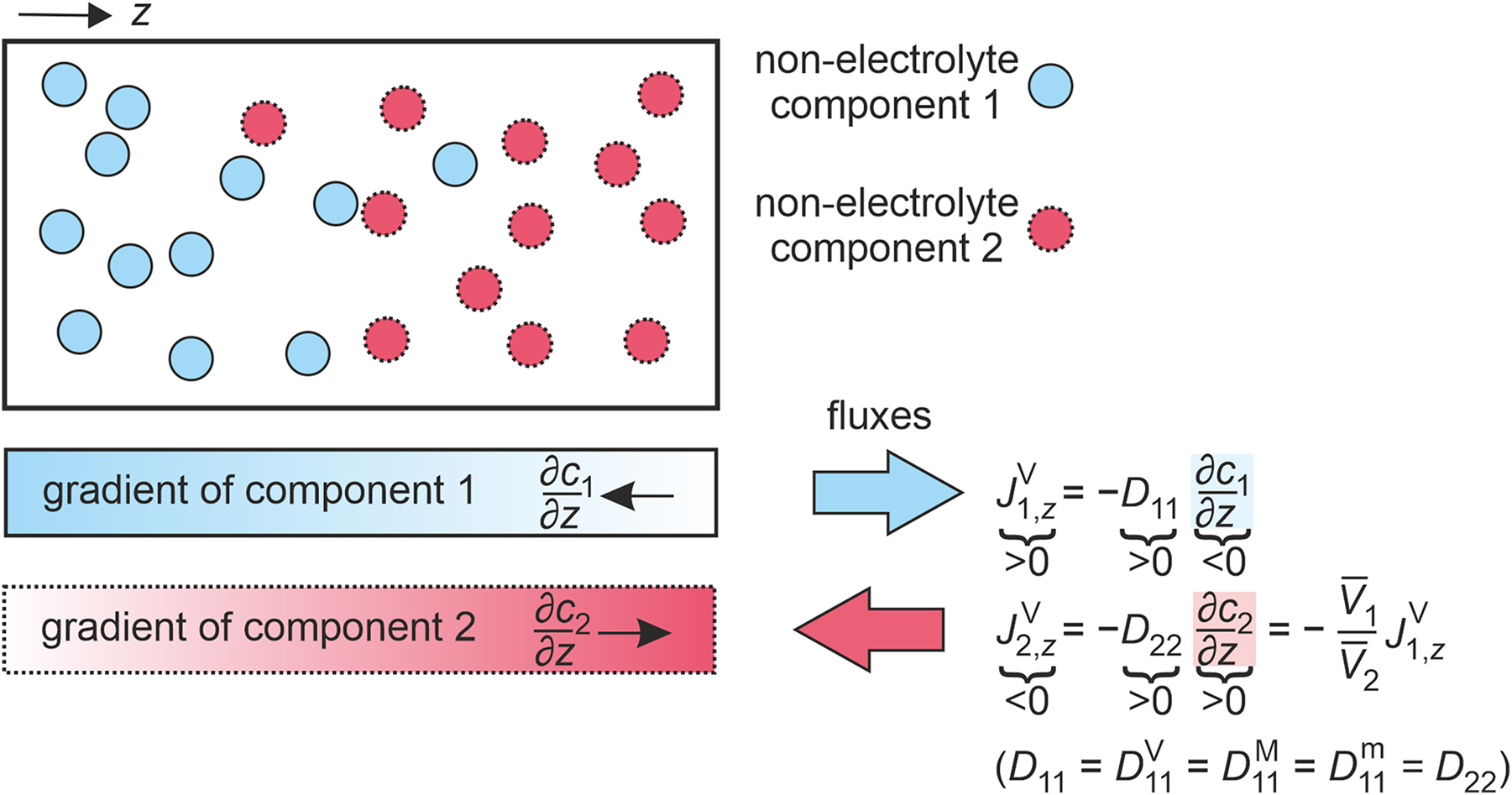
Illustration of the gradients and fluxes in a binary non-electrolyte mixture consisting of components 1 and 2 at an instant of time. Additionally, the relationships between the one-dimensional amount fluxes in the volume-averaged reference frame
In this case, the diffusion process is entirely described by one independent diffusive flux and one independent driving force for diffusion. As a result, a single Fick diffusion coefficient characterizes diffusive mass transport in a binary mixture. The generalized expressions of Fick’s law given in Eqs. (2)–(4) in the volume-, amount-, and mass-averaged reference frames simplify to
For a binary mixture, the Fick diffusion coefficients obtained in the three addressed reference frames are identical, i.e.,
Equation (25) does not contain an averaged mixture velocity so that D 11 does not depend on the reference frame and its superscript can be omitted.
We recommend the use of D 11 to identify the Fick diffusion coefficient, which is also referred to as the interdiffusion coefficient, in a binary mixture to be consistent with the terminology for the Fick diffusion coefficients of n-component mixtures that are discussed in the next section. This differs from the terminology adopted by many authors in the literature, where, for example, D 12 or D AB can be found, but is essential if consistency with multicomponent mixtures is to be retained.
In addition to the above reference frames, which are often used in diffusion research, further reference frames can be adopted according to the nature of the problem studied. An example is the solvent velocity as the reference frame. 17 , 18 The Fick diffusion coefficient in this reference frame is not identical with those obtained in the volume-, amount-, or mass-averaged reference frames, except for conditions in the infinite dilution limit, i.e., when the concentration of one of the two components is very small. Thus, care needs to be taken when comparing Fick diffusion coefficient data from other reference frames with those obtained in volume-, amount-, or mass-averaged reference frames.
For a binary mixture according to Maxwell–Stefan theory, Eq. (19) reduces to
where the thermodynamic factor Γ 11 is a scalar quantity given by Eq. (20) as
A comparison of Eq. (23) and (26) yields the relation between the Fick and Maxwell–Stefan diffusion coefficients of a binary mixture,
For ideal mixtures and in both infinite dilution limits, Γ 11 = 1 holds so that D 11 = Đ 12. In other situations, Γ 11 can be derived from composition-dependent activity coefficient data. Alternatively, it can be obtained from Kirkwood–Buff integrals, 19 , 20 which are directly accessible by molecular simulation. 21 , 22
Self- and tracer-diffusion coefficients.
In addition to the above-mentioned transport diffusion coefficients, self- and tracer-diffusion coefficients can be defined. While these diffusion coefficients do not qualify as transport properties, they can be employed to describe diffusive mass transport in certain cases. The self-diffusion coefficient, which is sometimes referred to as intra-diffusion coefficient, of component i, D
i
, is a measure of its molecular mobility within either a pure substance or a mixture. Self-diffusion coefficients of the components in the mixture depend on the composition. In the infinite dilution limit of component 1, i.e., x
1 → 0, D
1 converges to D
11 and Đ
12. By analogy, D
2 approaches D
11 and Đ
12 in the infinite dilution limit of component 2, i.e., x
2 → 0. These relations can also be derived from the Green–Kubo formalism for Đ
12.
23
,
24
In the infinite dilution limit x
i
→ 0, the Fick diffusion coefficient is referred to as the tracer-diffusion coefficient

Self-diffusion coefficients D
i
, tracer-diffusion coefficients
2.2 Ternary mixtures
This section provides definitions and terminology for diffusion coefficients of ternary systems where n = 3. A ternary non-electrolyte mixture consisting of the components 1, 2, and 3 is illustrated in Fig. 3. An example for such a mixture would be the ternary mixture of ethanol, n-hexane, and acetone. n
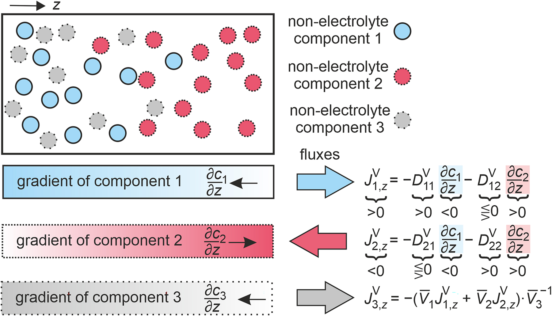
Illustration of gradients and fluxes in a ternary non-electrolyte mixture consisting of components 1, 2, and 3 at an instant of time. Additionally, the relationships between the one-dimensional amount fluxes in the volume-averaged reference frame
As in the previous section, only mixtures consisting of non-electrolyte components are considered so that the number of species and components is identical. For ternary mixtures, there are two independent diffusive fluxes. Hence, four different Fick diffusion coefficients are required for their characterization. According to Fick’s law, the fluxes can be expressed in the volume-, amount-, and mass-averaged reference frames as
The diagonal elements of the Fick diffusion coefficient matrix D 11 and D 22 characterize the diffusive flux of components 1 and 2 due to the gradients of their own concentration, amount fraction, or mass fraction, whereas the off-diagonal elements D 12 and D 21 characterize the diffusive fluxes of these components due to the corresponding gradients of the other independent component. The Fick diffusion coefficient matrix is generally asymmetric and its numerical values depend on the reference frame and component order, as discussed below.
Unlike Fick diffusion coefficient matrices, Maxwell–Stefan diffusion coefficient matrices are independent of reference frame and component order. They are symmetric, i.e., Đ ij = Đ ji , so that only three coefficients are required to describe the diffusive fluxes in a ternary mixture. Akin to binary mixtures, Maxwell–Stefan and Fick diffusion coefficient matrices are linked via the thermodynamic factor given as a 2 × 2 matrix. For a ternary mixture, Maxwell–Stefan theory reads in explicit matrix form
where the four elements of the 2 × 2 diffusion coefficient matrix B are given by
Self- and tracer-diffusion coefficients. For multicomponent mixtures, self- and tracer-diffusion coefficients can also be defined. While the tracer-diffusion coefficient has a single value for a given temperature and pressure pair in the case of a binary mixture, it depends further on the relative amount of the remaining two components in the case of a ternary mixture.
If the amount fraction of one of the first two components (i ≠ n) vanishes, i.e., x i → 0, the following limits of some elements of the Fick diffusion coefficient matrix of a ternary mixture are reached,
where
2.3 Transformation between reference frames
In the following, the transformation of the Fick diffusion coefficient matrix from one reference frame into another is explained for non-electrolyte systems. Fick diffusion coefficients obtained experimentally are often given in the volume-averaged reference frame, while the amount-averaged reference frame is the natural choice for Maxwell–Stefan theory and molecular simulation. To compare different approaches, the relation between the Fick diffusion coefficients in different reference frames is important. The Fick diffusion coefficient matrix in the amount-averaged reference frame D M can be transformed into its form in the mass-averaged reference frame D m employing 11 , 25
where [ x ] and [ w ] are the diagonal matrices of the amount and mass fractions x i and w i , respectively.
The elements of the transformation matrices B mM and B Mm are given by
where the subscript n refers to the reference component.
Similarly, D M can be transformed into the Fick diffusion coefficient matrix in the volume-averaged reference frame D V with
where the amount-specific volume of the mixture V
M is the sum of the partial amount-specific, or molar, volumes, weighted by the amount fractions
The relation between the reference-invariant Fick diffusion coefficient matrix D and the ones in the mass-, amount-, and volume-averaged reference frames reads 12
Expressing measured and simulated diffusivity data via frame-independent diffusion coefficients has several advantages, such as an easier comparison between different data sets and a larger data base for testing and developing of models and predictions. Therefore, it is recommended to always publish the results in the form of frame-independent diffusivities, D , if possible.
2.4 Variation of the component order for non-electrolyte systems
Diffusive fluxes in multicomponent mixtures do not physically depend on the component order, but the values of the Fick diffusion coefficients do, because only n − 1 fluxes are formulated explicitly. The amount flux of the reference component i = n is obtained from the mass conservation condition
for i, j ≠ n. Therein,
In case the reference component is changed from n = 3 to a = 1, the diffusive fluxes of the two components 2 and 3 are given by
Here, it should be mentioned again that there is no virtue in recommending any particular choice of a reference component. The reference component and the order of the components can be chosen arbitrarily, and the resulting expressions will always give a full description of the diffusive mass transport.
3 Electrolyte systems
Following the definition given by Newman and Thomas-Alyea, 26 an electrolyte can be defined as follows: “An electrolyte is a material in which the mobile species are ions and free movement of electrons is blocked. Ionic conductors include molten salts, dissociated salts in solution, and some ionic solids. In an ionic conductor, neutral salts are found to be dissociated into their component ions. We use the term species to refer to ions as well as neutral molecular components that do not dissociate.” Therefore, the term “electrolyte system” refers to any system that contains mobile ions. Such an electrolyte system can contain only one component, e.g., a pure ionic liquid, or multiple components, which are then referred to as electrolyte mixtures. Here, it should be noted that an electrolyte mixture can contain multiple electrolyte components, such as a mixture of two ionic liquids, or one or more electrolytes dissolved in one or more non-electrolyte components, such as a salt dissolved in an organic solvent.
Mass transport in the bulk of electrolyte fluids can take place owing to diffusion and migration. In this work, only the diffusive mass transport owing to a gradient of the (electro)chemical potential in the absence of an electric field at constant temperature and pressure is considered. For electrolyte mixtures, this case is often referred to as the ‘pure diffusion problem’. For an overview about the design of an experiment to access diffusion coefficients in electrolyte systems, the reader is referred to the work of Newman and colleagues. 5 , 33
3.1 Binary mixtures
Just as a binary non-electrolyte mixture, a binary electrolyte mixture consists of two components, but it contains at least one electrolyte component, which dissociates into cations and anions in solution. As a result, the mixture consists of at least three species.
3.1.1 Binary electrolyte mixtures consisting of an electrolyte component and a non-electrolyte component
In the following, the two components of the binary electrolyte mixture are the electrolyte component or salt (component 1) and non-electrolyte component (component 2). Furthermore, it is assumed that the electrolyte component fully dissociates into cations and anions, 17 , 26 , 27
Here, υ 1+ and υ 1− are the stoichiometric coefficients of the cation and anion, while z 1+ and z 1− are their charge numbers. Furthermore, charge conservation demands υ 1+ z 1+ + υ 1− z 1− = 0. 17 As a result, three different species, namely, cation 1+, anion 1−, and non-electrolyte component 2, constitute the mixture. Figure 4 illustrates such a binary mixture exemplarily. An example for such a mixture would be sodium chloride [Na]+[Cl]− dissolved in acetonitrile.
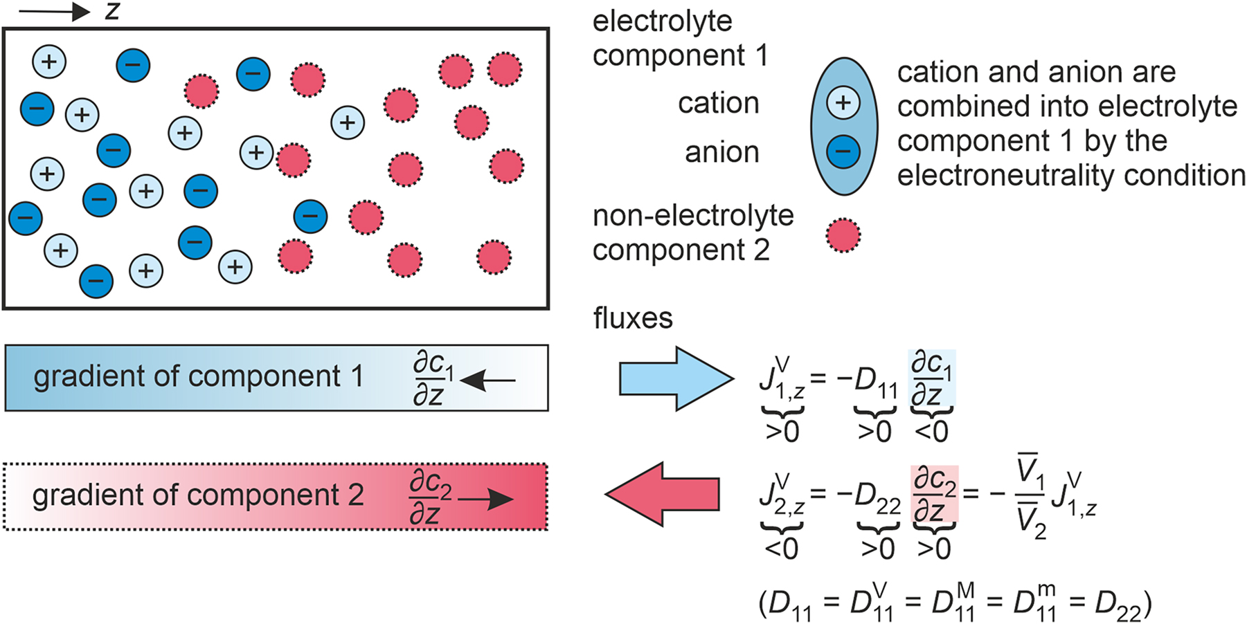
Illustration of gradients and fluxes in a binary electrolyte mixture consisting of an electrolyte component 1, dissociated into cations 1+ and anions 1−, and a non-electrolyte component 2 at an instant of time. Additionally, the relationships between the one-dimensional amount fluxes in the volume-averaged reference frame
With respect to the positive and negative charges in the bulk, the electroneutrality condition also needs to be satisfied, which leads to 26 , 28
As a result, the propagation and the diffusive fluxes of the ions are related. Under these conditions, the net current vanishes, and cations and anions have a coupled motion. 17 , 27 , 29 This constraint stipulates an additional condition, which needs to be satisfied in addition to the constraints on the different reference frames in the general case of a non-electrolyte mixture. In this context, it can be shown that the velocity of the cations u 1+ and the velocity of the anions u 1− are identical, cf. Section S1 in the Supporting information. Therefore, their velocities can be described by u 1+ = u 1− = u 1, where u 1 represents the velocity of the electrolyte component as a whole. This means that cations and anions diffuse like a single non-electrolyte component in the mixture. 17 As a result, diffusion in a binary electrolyte mixture can be treated like diffusion in a binary non-electrolyte mixture and the flux expressions can be written either for the electrolyte or non-electrolyte component. 27 , 30
Diffusive mass transport according to Fick. In binary electrolyte mixtures, there is only one independent diffusive flux 31 and one independent chemical potential or concentration gradient 11 as the driving force for diffusion. Thus, a single Fick diffusion coefficient D 11 characterizes the diffusive mass transport.
In the volume-averaged reference frame, the gradient of the concentration of the electrolyte component as a whole is used to express the driving force for its amount flux according to 27
Therein,
Similarly, c 1 is related to the concentration of the cation c 1+ and the anion c 1− according to 26
Combining Eqs. (47)–(49), the amount fluxes for the cations and anions can be expressed explicitly as
The volume-averaged reference velocity u V is given by
Since partial amount-specific volumes, also referred to as partial molar volumes, of the individual ionic species, namely, the one of the cation
In the amount-averaged reference frame, the amount flux of component 1 is
Here, c = c 1+ + c 1− + c 2 and x 1 = c 1/c, where c 1 is defined according to Eq. (49). 26 Furthermore, x 1 can also be related to the amount fraction of the cation or the anion by 32 x 1 = x 1+/υ 1+ = x 1−/υ 1− and u M defines the amount-averaged reference velocity according to u M = x 1+ u 1+ + x 1− u 1− + x 2 u 2. Based on the relation
the amount fluxes of the cation and the anion can be expressed as
The closing condition
In the mass-averaged reference frame, the mass flux of component 1 is
The mass density of the mixture is ρ = ρ 1+ + ρ 1− + ρ 2, where ρ i is the mass density of the respective species. The mass fraction of the electrolyte component is given by 26 w 1 = (ρ 1+ + ρ 1−)/ρ and u m defines the mass-averaged reference velocity given by u m = w 1+ u 1+ + w 1− u 1− + w 2 u 2, where w i = ρ i /ρ is the mass fraction of species i in the mixture. The mass fluxes of the cations and the anions may further be expressed as
The constraint
In binary electrolyte mixtures, the Fick diffusion coefficient is independent of a reference velocity frame,
However, this difference vanishes in the infinite dilution limit of the solute, where
Diffusive mass transport according to Maxwell-Stefan theory. For an electrolyte mixture, the relationship between the driving force, i.e., the (electro)chemical potential gradient, and the friction forces expressed by the relative velocity of two components or species must be specified for the constituent species. As in the previous section, similar notations are adopted for the cation with 1+, for the anion with 1−, and for the non-electrolyte component with 2. Thus, for the three species k at constant temperature and pressure, Eq. (15) becomes
Here, μ i stands for the electrochemical potential of ionic species or for the chemical potential of electroneutral components. There are three independent Maxwell–Stefan diffusion coefficients among the three species, namely, Đ 1+,1−, Đ 1+,2, and Đ 1−,2. Owing to the electroneutrality condition in the absence of an external electric field, only one independent diffusive flux is present and, therefore, only one Maxwell–Stefan diffusion coefficient is required to describe the diffusive mass flux. This component-based Maxwell–Stefan diffusion coefficient Đ 12 can be derived from the three species-based Maxwell–Stefan diffusion coefficients according to 26
The flux expression for the electrolyte component as a whole can be written as
Thus, Đ 12 can be related to D 11 via the thermodynamic factor Γ 11 by
The required Γ 11 can be determined from the mean activity coefficient of the electrolyte component γ 1± or from the activity coefficient of the non-electrolyte component γ 2 via 32
Here, γ
1± is related to the activity coefficient of the cation and the anion according to
Self-diffusion coefficients D i . For a binary electrolyte mixture, three self-diffusion coefficients D i can be defined. In the infinite dilution limit of the electrolyte component 1, the self-diffusion coefficient of the cations D 1+ and of the anion D 1− can be related to Đ 12 and D 11 by
Furthermore, the self-diffusion coefficient of the non-electrolyte component D
2 becomes equal to the self-diffusion coefficient of the pure component 2. Approaching the infinite dilution limit of the electrolyte component 1, two tracer-diffusion coefficients can be found,
Self-diffusion coefficients D
i
, tracer-diffusion coefficients
3.1.2 Binary electrolyte mixtures consisting of three ionic species
Another type of a binary electrolyte mixture consists of two electrolyte components that share a common ion, i.e. either the same cation or the same anion. In this section, the latter case is taken as an example. It is assumed that the two electrolyte components fully dissociate according to
For the anion species (−), 1 or 2 could be used to represent the component, where 1 is employed here. Figure 6 illustrates such a binary mixture exemplarily. An example for such a mixture would be lithium bis(trifluoromethylsulfonyl)imide [Li]+[NTf2]− dissolved in the ionic liquid 1-ethyl-3-methylimidazolium bis(trifluoromethylsulfonyl)imide [EMIm]+[NTf2]−, where the anion [NTf2]− represents the common ion.
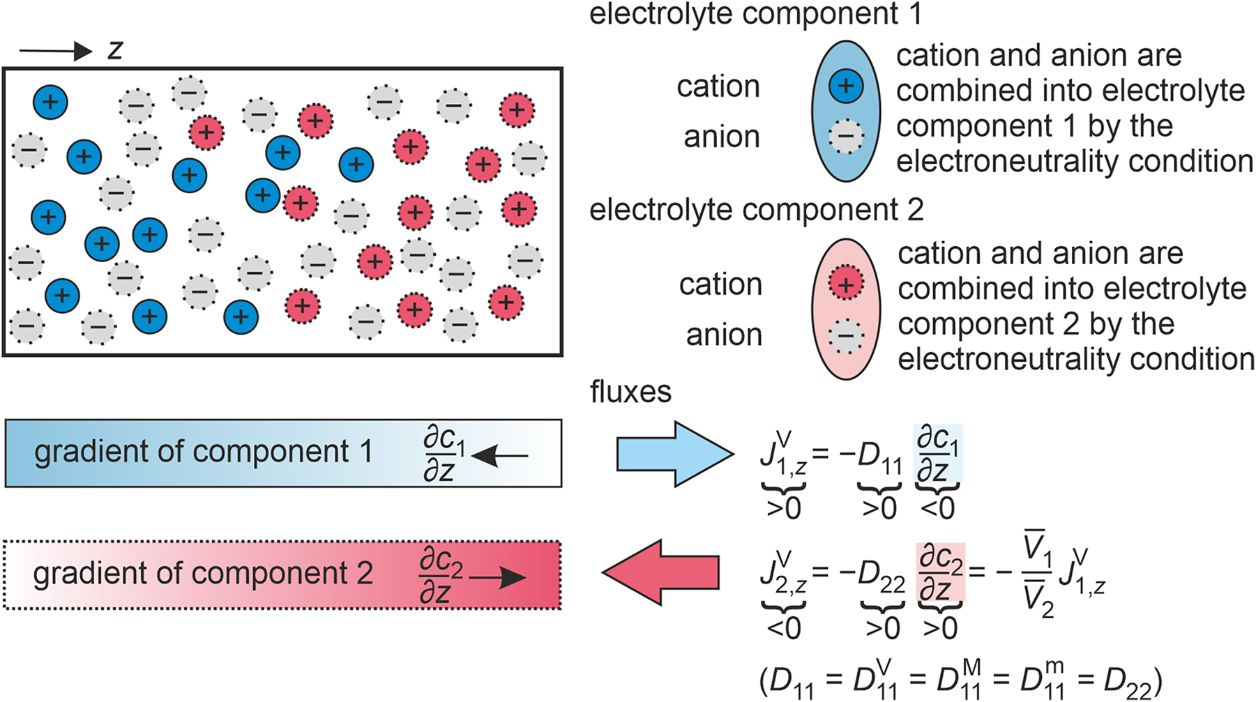
Illustration of gradients and fluxes in a binary electrolyte mixture consisting of two electrolyte components 1 and 2, which share a common anion, at an instant of time. Additionally, the relationships between the one-dimensional amount fluxes in the volume-averaged reference frame
Charge conservation upon dissociation of electrolyte components demands υ 1+ z 1+ + υ 1− z 1− = 0 and υ 2+ z 2+ + υ 2− z 1− = 0. Because of the common anion of both components, the mixture consists of the three species 1+, 2+, and 1−, while there is no solvent component.
Diffusive mass transport according to Fick. As for the previously discussed binary electrolyte mixture, only one independent driving force and one independent diffusive flux exist for binary electrolyte mixtures consisting of three ionic species. Thus, diffusive mass transport is characterized by a single Fick diffusion coefficient. Furthermore, volume-, amount-, or mass-averaged reference frames can be applied for the description of the diffusive fluxes. The required expressions for the diffusive fluxes in the volume-, amount-, or mass-averaged reference frames can be found in Ref. 34]. In the following, only the flux expressions for species 1+ are given as a representative example. In the volume-averaged reference frame, the amount flux of species 1+ is 34
where
u
V is the reference velocity, which is defined as
In the amount-averaged reference frame, the amount flux of species 1+ is written in the form 34
where υ
2 is defined as υ
2 = υ
2+ + υ
2−. It is important to note that Eq. (69) was derived using a different definition of the amount fraction of the electrolyte component 1. In Pollard and Newman,
34
the amount fraction of the electrolyte component 1,
In the mass-averaged reference frame, the mass flux of species 1+ is 34
Here, w 1+ is the mass fraction of species 1+, defined as w 1+ = ρ 1+/ρ, and u m is the reference velocity according to u m = w 1+ u 1+ + w 2+ u 2+ + w 1− u 1−.
The three discussed reference frames lead to an identical Fick diffusion coefficient,
Diffusive mass transport according to the Maxwell-Stefan theory. For the three species in a mixture consisting of two electrolyte components sharing a common ion, Maxwell–Stefan theory defines three independent species-based Maxwell–Stefan diffusion coefficients Đ 1+,1−, Đ 1+,2+, and Đ 2+,1− when the anion is shared. The three Maxwell–Stefan diffusion coefficients result in one component-based Maxwell–Stefan diffusion coefficient Đ 12, which fully describes the diffusive mass transport in the absence of an external electric field according to 34
A corresponding equation can also be written for a shared cation. For a common anion, Đ
12 is related to the Fick diffusion coefficient
Here, γ 1 is the activity coefficient of the electrolyte component 1 disregarding its dissociation.
Self-diffusion coefficients D
i
.
For the case of a shared anion, three self-diffusion coefficients D
1+, D
2+, and D
1− can be defined. In the infinite dilution limit of an electrolyte component, these three D
i
may be related to Đ
12 = D
11 via the multi-component Darken approximation.
35
Note that the shared ion in the considered systems is never at infinite dilution. In the infinite dilution limit, D
i
of an unshared ion i is also referred to as the tracer-diffusion coefficient
3.2 Multi-component electrolyte mixtures
In an n-component electrolyte mixture, k different species with k ≥ n + 1 exist. In the absence of an external electric field, k – 2 independent diffusive fluxes 31 and k − 2 independent chemical potential or concentration gradients 11 can be defined. This entails a Fick diffusion coefficient matrix of dimension (k – 2) × (k – 2) and k × (k – 1)/2 species-based Maxwell–Stefan diffusion coefficients. In the following, the treatment of diffusion problems in a multicomponent electrolyte mixture is highlighted exemplarily for a ternary electrolyte mixture containing a single electrolyte component.
3.2.1 Ternary electrolyte mixture consisting of an electrolyte and two non-electrolyte components
Here, the electrolyte is considered to be component 1, which fully dissociates according to
Thus, the four different species present in the mixture are identified with 1+, 1−, 2, and 3. Figure 7 illustrates such a ternary mixture exemplarily. An example for such a mixture would be sodium chloride [Na]+[Cl]− dissolved in a mixture of acetonitrile and diethyl carbonate.

Illustration of gradients and fluxes in a ternary electrolyte mixture consisting of an electrolyte component 1, dissociated into cations 1+ and anions 1−, and the non-electrolyte components 2 and 3 at an instant of time. Additionally, the relationships between the one-dimensional amount fluxes in the volume-averaged reference frame
In the following, the diffusive mass transport is expressed via Fick’s law and Maxwell–Stefan theory.
Diffusive mass transport according to Fick. Owing to the electroneutrality condition, the diffusive fluxes of the ions are again coupled. As a result, there are two independent diffusive fluxes and two independent chemical potential or concentration gradients acting as driving forces. The cation and the anion can be treated together as a single electroneutral component and the fluxes can be described with the corresponding equations for ternary non-electrolyte mixtures according to Fick’s law. 36 In the volume-averaged reference frame, the amount fluxes of components 1 and 2 can be expressed as
where c
1 and c
2 are the concentrations of the electrolyte component 1 and the non-electrolyte component 2. Here, c
1 is related to the concentration of the cations and anions according to
The amount flux of the non-electrolyte component 3 is then given by the closing condition
In the amount-averaged reference frame, the amount fraction gradients are assumed as the driving force. Like for binary electrolyte mixtures,
26
the amount fraction of the electrolyte component i in the mixture is x
i
= c
i
/c, where c is the total concentration according to c = c
1+ + c
1− + c
2 + c
3. Note that the amount fraction of the electrolyte component is related to the amount fractions of its cation and anion via
Here, u M is the amount-averaged reference velocity given by u M = x 1+ u 1+ + x 1− u 1− + x 2 u 2 + x 3 u 3.
In the mass-averaged reference frame, the mass fluxes of components 1 and 2 can be written as
Therein, w i = ρ i /ρ is the mass fraction of component i with i = 1 or 2, whereas ρ i is the mass density of component i and ρ is the total mass density of the mixture according to ρ = ρ 1+ + ρ 1− + ρ 2 + ρ 3. Note that the mass fraction of the electrolyte component 1, w 1, is related to the mass fractions of the cation and the anion by w 1 = w 1+ + w 1− and u m is the mass-averaged reference velocity given by u m = w 1+ u 1+ + w 1− u 1− + w 2 u 2 + w 3 u 3.
In addition to the aforementioned reference frames, the solvent velocity has also been applied as the reference velocity in the literature. 36 Furthermore, the transformation of the Fick diffusion coefficient matrix from the volume-averaged reference frame to the solvent-velocity reference frame and vice versa has been outlined in the literature. 36
Transformation between reference frames. The Fick diffusion coefficient matrices in the volume-, amount-, and mass-averaged reference frames can be represented by D V, D M, and D m, respectively. These matrices are of dimension 2 × 2 and are in general not symmetric. Again, the numerical values of their entries depend on the reference frame and the component order. To allow for the comparison of a Fick diffusion coefficient matrix given in one reference frame to that given in another reference frame, a transformation is necessary. To obtain the transformation matrices, we followed the procedure proposed by Ortiz de Zárate and Sengers, 12 , 39 where details are provided in Section S3 of the Supporting information. For this transformation, the relationships between diffusive amount or mass fluxes and the driving force gradients in the different reference frames are required. This can be achieved by introducing the matrices
Matrix W contains the mass fractions of the components according to w i = ρ i /ρ, where the mass density of the mixture ρ is given by ρ = ρ 1+ + ρ 1− + ρ 2 + ρ 3, and Φ contains the amount fractions x i and the volume fractions ϕ i . Here, x i = c i /c and ϕ i = V¯ i c i . Matrix X contains stoichiometrically weighted amount fractions x i* that are defined as x 1* = υ 1 x 1 for the electrolyte component 1 and x 2* = x 2 for the non-electrolyte component 2. With these stoichiometrically weighted amount fractions, the general structure of X remains similar to that of a non-electrolyte ternary mixture. 12 Finally, the Fick diffusion coefficient matrix in the amount-averaged reference frame D M can be transformed to the one in the mass-averaged reference frame D m via
The transformation from D M into D V is
Diffusive mass transport according to the Maxwell-Stefan theory. Using Maxwell–Stefan theory, 13 , 14 the corresponding equations must be written for the involved species. For an ionic species i, the driving force for diffusive mass transport is the electrochemical potential gradient ∇μ i . For a non-electrolyte component i, it is the chemical potential gradient of that component indicated by the same symbol. The resulting Maxwell–Stefan diffusion coefficient matrix can be related to the Fick diffusion coefficient matrix in the amount-averaged reference frame. However, to the best of our knowledge, the relationship between the governing equations using the Maxwell–Stefan theory and Fick’s law for a ternary or multicomponent electrolyte mixture has not been presented in the literature so far. Thus, these equations were developed within this work. Since such a relation can easily be extended to a general multicomponent mixture, we outline this relationship for a n-component electrolyte mixture containing a single electrolyte component. In the following, the electrolyte component is referred to as component 1. The present species are 1+, 1−, 2, 3, …, n, and we consider k = n + 1 as the number of species to distinguish between the species- and component-based relations. For a k-species electrolyte system, this yields
where the property
which states that the velocity of both ion types in the mixture is identical, so that the velocity of the electrolyte component 1 as a whole can be referred to as u 1. Note that the expression for the current flux is independent of the reference frame, 17 , 26 so that no ambiguity arises. Owing to the dissociation of the electrolyte component, its amount fraction is x 1 = x 1+/υ 1+ = x 1−/υ 1−. Furthermore, it is practical to adopt the stoichiometrically weighted amount fractions according to x 1* = υ 1 x 1 for the electrolyte component 1 and keep x i* = x i for the non-electrolyte components. Such a modification results in a simplification of the resulting expressions, cf. Section S3 of the Supporting information.
With the relation for the velocities of the ions in Eq. (86) and the stoichiometrically weighted amount fractions, the chemical potential of the electrolyte component 26 μ 1 = υ 1+ μ 1+ + υ 1− μ 1− can be introduced so that Maxwell–Stefan theory can be expressed by
where α 1 = 1/υ 1 and
Furthermore, it follows that
where Đ 1,j is the component-based Maxwell–Stefan diffusion coefficient between the electrolyte component 1 and the non-electrolyte component j. Note that in Eq. (87), the subscript 1 in K 1,j is attributed to the electrolyte component and the subscript j with j ≠ 1 in K 1,j represents the non-electrolyte component j. Similarly, Eq. (85) can be written for a non-electrolyte component i in the simplified form
where α i = 1 in this case. While K i,1 is given by Eq. (88), K i,j for i and j ≠ 1 is given by
Consequently, the Maxwell–Stefan expressions for the species can be generalized to a component-wise representation, which, for an arbitrary component i in the mixture, can be written as
Here, the term α i is maintained to retain the generality of the expressions, where α 1 = 1/υ 1 for the electrolyte component 1 and α i = 1 otherwise. The properties K i,j are given by Eqs. (88) and (91). Note that the set of equations according to Maxwell–Stefan theory now takes a similar form as that of a n-component non-electrolyte mixture. Furthermore, only n − 1 independent equations can be written from Eq. (92) under diffusion problem conditions. Following the procedure suggested by Taylor and Krishna, 11 Eq. (92) can be rewritten by eliminating the term for component n with the amount-averaged reference velocity u M to obtain
where
Furthermore, Eq. (93) can be rearranged to
The amount fraction x
1 is convenient for the electrolyte component. With that choice, diffusive amount fluxes of the cations and the anions can be obtained straightforwardly. For that purpose, x
i*
needs to be transformed back to x
i
via x
i*
= υ1
x
1 for the electrolyte component and x
i*
= x
i
for the non-electrolyte components. In addition, the chemical potential of the electrolyte component is usually expressed via its mean activity coefficient γ
1± according to
where M is a diagonal matrix with M 11 = υ 1 −1 , M ii,i≠1 = 1, and M ij,i≠j = 0, while Γ is the thermodynamic factor matrix. The respective Fick diffusion coefficient matrix in the amount-averaged reference frame D M can now be related to the Maxwell–Stefan diffusion coefficient matrix according to
where the matrix B contains the Maxwell–Stefan diffusion coefficients.
Equation (97) can be compared with expressions from the literature for a binary electrolyte mixture containing a single electrolyte component. Here, it can easily be shown that it is identical with the one given in Section 3.1.1 in the amount-averaged reference frame. In addition, the resulting matrix with the elements Γ ij based on the amount fraction of the electrolyte component is essentially the one given by Liu and Monroe 32 and can be simplified to the one defined by Newman in terms of molalities. 26
For a ternary mixture, Eq. (97) takes the form
Here, the diagonal elements of matrix B are
and the corresponding off-diagonal elements are
D M is related to the Maxwell–Stefan diffusion coefficients by
3.2.2 Other types of ternary electrolyte mixtures
In addition to the ternary electrolyte mixture containing a single electrolyte component, we would like to highlight the remaining two types of ternary mixtures, which are
a mixture consisting of one non-electrolyte component and two electrolyte components that share one common ion and
a mixture consisting of three electrolyte components, where all three share one common ion.
Assuming full ion dissociation, these two types of mixtures contain four different species. Owing to the electroneutrality condition, there are only two independent chemical potential gradients and two independent diffusive mass fluxes in the absence of an external electric field. Thus, the corresponding Fick diffusion coefficient matrix is of dimension 2 × 2. For type (a) mixtures, the corresponding flux expressions were outlined in the literature in the volume-averaged 41 and solvent-velocity reference frame. 30 Furthermore, the transformation of Fick diffusion coefficients from the volume-averaged to the solvent-velocity reference frame have been discussed in the literature. 30 However, the transformations of the Fick diffusion coefficient matrices between the volume-, amount-, and mass-averaged reference frames have so far not been discussed for this mixture type. For mixtures of type (b), the flux expressions are, to the best of our knowledge, not available in any reference frame. Also, the transformation of the Fick diffusion coefficient matrices between volume-, amount-, and mass-averaged reference frames as well as the relationship between the Fick and Maxwell–Stefan diffusion coefficient matrices are not available in the literature.
4 Conclusions
This work presents a compilation of the basic relationships that are necessary to describe molecular diffusive mass transport in non-electrolyte and electrolyte systems. Furthermore, it gives a clear guideline for the terminology of the associated diffusion coefficients. The work aims to resolve the ambiguity of the employed terminology for describing molecular mass transport and the related diffusion coefficients, which can often be found in the literature. It may help researchers working in the field of diffusion as a guideline.
Membership of sponsoring bodies
Membership of the IUPAC Physical and Biophysical Chemistry Division:
Division President: F. Separovic; Vice President: J. Frey; Past President: P. Metrangolo; Secretary: J. Luís Faria; Titular Members: M. Fall, H. N. Ghosh, R. Orinakova, A. Rodger, T. Wallington, M. Witko; Associate Members: K. Feng Chong, T. Frankcombe, E. Kazuma, M. Rissanen, I. Schapiro, I. Voets; National Representatives: N. Bregovic, C. Contini, K. Ghandi, E. V. Golubina, L. Liu, P. Nelson, V. Parasuk, I. A. Pasti, B. Rangelov, C.-L. Wang; Emeritus Fellows: T. Cvitas, R. Weir
Funding source: International Union of Pure and Applied Chemistry
Award Identifier / Grant number: Project No.: 2014-010-1-100
-
Research ethics: Not applicable.
-
Informed consent: Not applicable.
-
Author contributions: All authors have accepted responsibility for the entire content of this manuscript and approved its submission.
-
Use of Large Language Models, AI and Machine Learning Tools: None declared.
-
Conflict of interest: The authors state no conflict of interest.
-
Research funding: This report was prepared under the framework of IUPAC Project 2014-010-1-100. Sponsoring body: IUPAC Physical and Biophysical Chemistry Division Committee.
-
Data availability: Not applicable.
References
1. Price, W. S. NMR Studies of Translational Motion: Principles and Applications; Cambridge University Press: Cambridge, 2009.10.1017/CBO9780511770487Search in Google Scholar
2. Bée, M. Quasielastic Neutron Scattering; Adam Hilger: Bristol, 1988.Search in Google Scholar
3. Cussler, E. L. Diffusion: Mass Transfer in Fluid Systems; Cambridge University Press: Cambridge, 2009.10.1017/CBO9780511805134Search in Google Scholar
4. Tyrrell, H. J. V.; Harris, K. R. Diffusion in Liquids: A Theoretical and Experimental Study; Butterworth-Heinemann: Oxford, 2013.Search in Google Scholar
5. Newman, J.; Chapman, T. W. Restricted Diffusion in Binary Solutions. AIChE J. 1973, 19, 343–348. https://doi.org/10.1002/aic.690190220.Search in Google Scholar
6. Berne, B. J.; Pecora, R. Dynamic Light Scattering: With Applications to Chemistry, Biology, and Physics; Dover Publications: New York, 2000.Search in Google Scholar
7. Onsager, L. Reciprocal Relations in Irreversible Processes. I. Phys. Rev. 1931, 37, 405–426. https://doi.org/10.1103/PhysRev.37.405.Search in Google Scholar
8. Onsager, L. Reciprocal Relations in Irreversible Processes. II. Phys. Rev. 1931, 38, 2265–2279. https://doi.org/10.1103/PhysRev.38.2265.Search in Google Scholar
9. Anisimov, M. A.; Agayan, V. A.; Povodyrev, A. A.; Sengers, J. V.; Gorodetskii, E. E. Two-Exponential Decay of Dynamic Light Scattering in Near-Critical Fluid Mixtures. Phys. Rev. E 1998, 57, 1946–1961. https://doi.org/10.1103/PhysRevE.57.1946.Search in Google Scholar
10. Fick, A. Über Diffusion. Ann. Phys. 1855, 170, 59–86. https://doi.org/10.1002/andp.18551700105.Search in Google Scholar
11. Taylor, R.; Krishna, R. Multicomponent Mass Transfer; John Wiley & Sons: New York, 1993.Search in Google Scholar
12. Ortiz de Zárate, J. M.; Sengers, J. V. Frame-Invariant Fick Diffusion Matrices of Multicomponent Fluid Mixtures. Phys. Chem. Chem. Phys. 2020, 22, 17597–17604. https://doi.org/10.1039/D0CP01110J.Search in Google Scholar PubMed
13. Maxwell, J. C. On the Dynamical Theory of Gases. Phil. Trans. R. Soc. London I 1867, 157, 49–88.10.1098/rstl.1867.0004Search in Google Scholar
14. Stefan, J. Über das Gleichgewicht und die Bewegung, insbesondere die Diffusion von Gasgemengen. Sitzungsberichte der Mathematisch-Naturwissenschaftlichen Classe der Kaiserlichen Akademie der Wissenschaften Wien, 2te Abteilung 1871, 63, 63–124.Search in Google Scholar
15. Liu, X.; Martín-Calvo, A.; McGarrity, E.; Schnell, S. K.; Calero, S.; Simon, J. M.; Bedeaux, D.; Kjelstrup, S.; Bardow, A.; Vlugt, T. J. H. Fick Diffusion Coefficients in Ternary Liquid Systems from Equilibrium Molecular Dynamics Simulations. Ind. Eng. Chem. Res. 2012, 51, 10247–10258. https://doi.org/10.1021/ie301009v.Search in Google Scholar
16. Krishna, R.; van Baten, J. M. The Darken Relation for Multicomponent Diffusion in Liquid Mixtures of Linear Alkanes: An Investigation Using Molecular Dynamics (MD) Simulations. Ind. Eng. Chem. Res. 2005, 44, 6939–6947. https://doi.org/10.1021/ie050146c.Search in Google Scholar
17. Miller, D. G. Application of Irreversible Thermodynamics to Electrolyte Solutions. I. Determination of Ionic Transport Coefficients lij for Isothermal Vector Transport Processes in Binary Electrolyte Systems. J. Chem. Phys. 1966, 70, 2639–2659. https://doi.org/10.1021/j100880a033.Search in Google Scholar
18. Pecora, R. Dynamic Light Scattering: Applications of Photon Correlation Spectroscopy; Springer: New York, 1985.10.1007/978-1-4613-2389-1Search in Google Scholar
19. Kirkwood, J. G.; Buff, F. P. The Statistical Mechanical Theory of Solutions. I. J. Chem. Phys. 1951, 19, 774–777. https://doi.org/10.1063/1.1748352.Search in Google Scholar
20. Ben-Naim, A. Molecular Theory of Solutions; Oxford University Press: Oxford, 2006.10.1093/oso/9780199299690.001.0001Search in Google Scholar
21. Fingerhut, R.; Herres, G.; Vrabec, J. Thermodynamic Factor of Quaternary Mixtures from Kirkwood─Buff Integration. Mol. Phys. 2020, 118, e1643046. https://doi.org/10.1080/00268976.2019.1643046.Search in Google Scholar
22. Ruckenstein, E.; Shulgin, I. Entrainer Effect in Supercritical Mixtures. Fluid Phase Equilib. 2001, 180, 345–359. https://doi.org/10.1016/S0378-3812(01)00372-7.Search in Google Scholar
23. Green, M. S. Markoff Random Processes and the Statistical Mechanics of Time-Dependent Phenomena. II. Irreversible Processes in Fluids. J. Chem. Phys. 1954, 22, 398–413. https://doi.org/10.1063/1.1740082.Search in Google Scholar
24. Kubo, R. Statistical-Mechanical Theory of Irreversible Processes. I. General Theory and Simple Applications to Magnetic and Conduction Problems. J. Phys. Soc. Jpn. 1957, 12, 570–586. https://doi.org/10.1143/JPSJ.12.570.Search in Google Scholar
25. Miller, D. G. Some Comments on Multicomponent Diffusion: Negative Main Term Diffusion Coefficients, Second Law Constraints, Solvent Choices, and Reference Frame Transformations. J. Chem. Phys. 1986, 90, 1509–1519. https://doi.org/10.1021/j100399a010.Search in Google Scholar
26. Newman, J.; Thomas-Alyea, K. E. Electrochemical Systems, 3rd ed.; John Wiley & Sons: New Jersey, 2004.Search in Google Scholar
27. Chapman, T. W. The Transport Properties of Concentrated Electrolytic Solutions. Dissertation (UCRL-17768), University of California: Berkeley, 1967.Search in Google Scholar
28. Krishna, R.; Wesselingh, J. A. The Maxwell-Stefan Approach to Mass Transfer. Chem. Eng. Sci. 1997, 52, 861–911. https://doi.org/10.1016/S0009-2509(96)00458-7.Search in Google Scholar
29. Kirkwood, J. G.; Baldwin, R. L.; Dunlop, P. J.; Gosting, L. J.; Kegeles, G. Flow Equations and Frames of Reference for Isothermal Diffusion in Liquids. J. Chem. Phys. 1960, 33, 1505–1513. https://doi.org/10.1063/1.1731433.Search in Google Scholar
30. Miller, D. G. Application of Irreversible Thermodynamics to Electrolyte Solutions. II. Ionic Coefficients lij for Isothermal Vector Transport Processes in Ternary Systems. J. Chem. Phys. 1967, 71, 616–632. https://doi.org/10.1021/j100862a024.Search in Google Scholar
31. Leaist, D. G. Electrolyte Diffusion in Multicomponent Solutions. Dissertation (8110046), Yale University: New Haven, 1980.Search in Google Scholar
32. Liu, J.; Monroe, C. W. Solute-Volume Effects in Electrolyte Transport. Electrochim. Acta 2014, 135, 447–460. https://doi.org/10.1016/j.electacta.2014.05.009.Search in Google Scholar
33. Stewart, S. G.; Newman, J. The Use of UV/vis Absorption to Measure Diffusion Coefficients in LiPF6 Electrolytic Solutions. J. Electrochem. Soc. 2008, 155, F13–F16. https://doi.org/10.1149/1.2801378.Search in Google Scholar
34. Pollard, R.; Newman, J. Transport Equations for a Mixture of Two Binary Molten Salts in a Porous Electrode. J. Electrochem. Soc. 1979, 126, 1713–1717. https://doi.org/10.1149/1.2128782.Search in Google Scholar
35. Liu, X.; Vlugt, T. J. H.; Bardow, A. Predictive Darken Equation for Maxwell–Stefan Diffusivities in Multicomponent Mixtures. Ind. Eng. Chem. Res. 2011, 50, 10350–10358. https://doi.org/10.1021/ie201008a.Search in Google Scholar
36. Woolf, L. A.; Miller, D. G.; Gosting, L. J. Isothermal Diffusion Measurements on the System H2O-Glycine-KCl at 25o; Tests of the Onsager Reciprocal Relation. J. Am. Chem. Soc. 1962, 84, 317–331. https://doi.org/10.1021/ja00862a001.Search in Google Scholar
37. Hao, L.; Leaist, D. G. Interdiffusion Without a Common Ion in Aqueous NaCl-MgSO4 and LiCl-NaOH Mixed Electrolytes. J. Solution Chem. 1995, 24, 523–535. https://doi.org/10.1007/BF00973204.Search in Google Scholar
38. Miller, D. G. Application of Irreversible Thermodynamics to Electrolyte Solutions. III. Equations for Isothermal Vector Transport Processes in n-Component Systems. J. Chem. Phys. 1967, 71, 3588–3592. https://doi.org/10.1021/j100870a037.Search in Google Scholar
39. Sengers, J. V. Mass Diffusion and Thermodiffusion in Multicomponent Fluid Mixtures. Int. J. Thermophys. 2022, 43, 1–10. https://doi.org/10.1007/s10765-022-02982-6.Search in Google Scholar
40. Bennion, D. N. Phenomena at a Gas-Electrode-Electrolyte Interface. Dissertation, University of California: Berkeley, 1957.Search in Google Scholar
41. Miller, D. G.; Ting, A. W.; Rard, J. A.; Eppstein, L. B. Ternary Diffusion Coefficients of the Brine Systems NaCl (0.5 M)-Na2SO4 (0.5 M)-H2O and NaCl (0.489 M)-MgCl2 (0.051 M)-H2O (Seawater Composition) at 25oC. Geochim. Cosmochim. Acta 1986, 50, 2397–2403. https://doi.org/10.1016/0016-7037(86)90021-9.Search in Google Scholar
Supplementary Material
This article contains supplementary material (https://doi.org/10.1515/pac-2024-0251).
© 2025 IUPAC & De Gruyter
This work is licensed under the Creative Commons Attribution-NonCommercial-NoDerivatives 4.0 International License.
Articles in the same Issue
- Frontmatter
- IUPAC Technical Reports
- Definitions and preferred symbols for mass diffusion coefficients in multicomponent fluid mixtures including electrolytes (IUPAC Technical Report)
- IUPAC/CITAC guide: interlaboratory comparison of categorical characteristics of a substance, material, or object (IUPAC Technical Report)
- Research Article
- Highly sensitive and eco-friendly molecular imprinting technique for determination of albumin