
Prediction of hypoglycaemia in subjects with type 1 diabetes during physical activity
-
Ornella Moro
 and
Giovanni Sebastiani
and
Giovanni Sebastiani

Abstract
Introduction
Practicing physical activity (PA) on a regular basis is an important support for people with type 1 diabetes (T1D). However, exercise may induce in them hypoglycaemic events during or after it. One major consequence of this is that, to limit this risk, many people with T1D tend to avoid performing PA. The availability of modern continuous glucose-monitoring (CGM) devices is potentially a great asset for reducing the chances of hypoglycaemia (HP) due to PA. Several algorithms have already been proposed to predict HP in subjects with T1D. However, not many of them are specifically focused on HP induced by exercise. Among those, many involve a large number of covariates making the applicability more difficult, and none uses CGM values available during the training session.
Objectives
We study the problem of predicting hypoglycaemia events in subjects with T1D during PA. The final aim is to produce algorithms enabling a person with T1D to perform a planned PA session without experiencing HP.
Method
One of the two algorithms we developed uses the CGM data in an initial part of a PA session. A parametric model is fitted to the data and then used to predict a possible HP during the remaining part of the session. Our second algorithm uses the CGM value at the start of a session. It also relies on statistical information about the average rate of decrease of the aforementioned model, as derived from a previously measured CGM data during PA. Then, the algorithm estimates the probability of HP during the planned PA session. Both algorithms have a very simple structure and therefore are of wide applicability.
Results
The application of the two algorithms to a very large dataset shows their very good ability to predict HP during PA in people with T1D.
Acronyms
- PA
-
Physical activity
- T1D
-
Type 1 diabetes
- CGM
-
Continuous glucose monitoring
- HP
-
Hypoglycaemia
- ROC
-
Receiver operating characteristic
- AUC
-
Area under the ROC curve
1 Introduction
Due to the needed insulin therapy, hypoglycaemia (HP) events are not rare for subjects with type 1 diabetes (T1D) when practicing physical activity (PA) [1,2]. Fear of hypoglycaemic events represents one of the major limitations for the practice of PA in people with T1D, although performing PA is proved to be a great asset to reduce long-term effects of high glucose concentration in tissues [3–5]. Several algorithms have been already developed to predict hypoglycaemic events in subjects with T1D performing or not PA. These algorithms use continuous glucose monitoring (CGM) data usually combined with some other covariates, e.g. carbohydrate intake and insulin on board. A recent review describes the main different types of algorithms that have been developed for this purpose [6]. However, among the 79 studies included in that review, only two of them are related to the prediction of HP specifically during PA [7,8]. Other interesting studies not included in that review have been published by Romero-Ugalde and colleagues [9] and by Bergford et al. [10]. Other possible approaches are related to novel machine learning and deep learning methods, in particular neural network (NN) [11–13]. However, most of these methods are not designed to detect PA-induced hypoglycaemia and require a very large quantity of data. Most important, they all use a number of CGM measurements larger than 10, while our algorithms at most use three measurements. Hence, these kind of models are not suited to solve our problem.
The first of the two aforementioned cited studies included in the review was published by Reddy and colleagues [7]. Here, the authors propose two different algorithms to predict HP during an aerobic PA session or immediately after it. The first algorithm is a decision tree classifier [14] using a minimum set of two covariates so that it can be widely applied. The two features used are the heart rate during exercise and the CGM value at the beginning of the session. To train the model, they use data previously collected during 154 sessions from 43 adults with T1D. The algorithm reaches an accuracy of about 80%. The second algorithm is based on random forest [15]. It uses 10 covariates, including the CGM value at the beginning of the PA session, some anthropometric data (sex, height, weight and BMI), heart rate and estimated energy expenditure during exercise, insulin on board, average amount of insulin injected per day, use of glucagon. Although the application of this algorithm is limited in respect to the first one, its accuracy is larger, reaching a value of about 87%. However, we notice that both algorithms do not use the CGM values during exercise.
In the second study cited earlier, Tyler et al. [8] present three different algorithms to predict glucose values and HP following or during aerobic PA sessions for people with T1D. In the first algorithm, the authors tailor a multivariate adaptive regression spline model introduced in a study of Friedman in 1991 [16]. This model is used to predict the minimum values of glucose concentration during the session and within 4 h after the end of it. The features used are the glucose value at the beginning of the session, the heart rate value 10 min before starting the exercise and the trend of CGM values in the 25 min prior the exercise. The model predicts HP during exercise with a sensitivity of 63% and an accuracy of 67%. For the prediction within the 4 h after the end of the session, the sensitivity decreases to 62%, while the accuracy reaches the 56%. The second algorithm is based on the logistic regression model presented by Breton [17] to predict HP during exercise. For this model, the variables included are the CGM value at the beginning of the session, the average CGM trend in the hour preceding exercise, the insulin on board at the beginning of the exercise and the total daily insulin requirement of the participant. In this case, the sensitivity achieved is 64% and the accuracy is the 61%. The last of the three algorithms is developed to predict the value of CGM at the end of the PA session. The sessions considered have an average duration of 40 min. The algorithm uses CGM values at the beginning of the training and at two times, a few tens of minutes before the start of the session. However, the used CGM values are obtained from the measured one through smoothing by means of a first-order auto-regressive model. The performance of this model are higher than the other two algorithms considered by these authors, with a sensitivity of 71% and an accuracy of 81%. The authors also include results from a personalized version, arriving at values of sensitivity and accuracy of about 76 and 83%, respectively. As mentioned earlier, these algorithms do not use CGM data during the exercise. In addition, the performances of these three algorithms are lower than those two proposed by Reddy and colleagues [7].
In the third cited study, Romero-Ugalde and colleagues [9] developed an algorithm that, in its final form, estimates the CGM at 30, 60 and 120 min after the start of a 30 min training. It uses CGM data and three other covariates, which are energy expenditure, insulin on board and carbohydrate on board, all the four up to 130 min before the start of the training. To predict the CGM value at a given time, an auto-regressive model of a certain order is used, with a time step of 10 min. The regression also includes the delayed effects of past sub-sequences of the three aforementioned covariates, with length (order) and delay depending on the covariate. To train and test the algorithm proposed, two different types of data were collected, denoted here as single PA protocol (SPA) and four PA protocol (FPA). In the SPA dataset, 34 subject performed a single PA session 3 h after lunch (happened at 12:00). Instead, for FPA, each of the 35 individuals enrolled trained for 3 consecutive days, 5 h after lunch (happened at 12:00). For FPA, an additional session was performed on the last day 3 h after the lunch, similarly as in SPA, for a total of four PA sessions for each individual. For each of the dataset, a sub-sample of 14 and 15 individuals, respectively, has been selected, which ensured a good quality of the collected signals. To estimate the model parameters, the prediction error has been minimized. Orders and delays are selected once within certain given intervals, by minimizing the Akaike final prediction error using SPA [18,19]. The performance was evaluated by estimating model parameters in two cases, at a population level or individually, respectively. In the first case, SPA data were used for training. Testing is then performed applying the estimated model only to the first session in the third day of the FPA data. However, best performance was obtained by individually estimating model parameters using the first, second and fourth sessions of FPA data and testing on the remaining third one. We notice that, beside the low sample dimension, we could not actually refer to prediction in this case. Indeed, the testing is performed to a session happening before the last one of the three used for parameter estimation. Furthermore, when performing parameter estimation only using one of the four FPA sessions available for each individual, the mean prediction error significantly increases.
The last study cited earlier is the most recent. Here, Bergford and colleagues [10] developed a different algorithm to predict HP during exercise for people with T1D. The algorithm presented is applied to a dataset consisting of around 500 subjects with several sessions each (total sessions 8,827). The original dataset is divided into two sub-samples to train the model (80% of participants) and to quantify the prediction performance (20%). The PA sessions last between 20 and 90 min and consist of aerobic, resistance and interval training types. Two algorithms are proposed, using two different sets of multiple predictors. Among these, the most important for both are the CGM value at start of training, rate of glucose change 15 min before the session, percent time with glucose
Our final goal here is to get people with T1D to perform a planned session of PA (or a maximal part of it) with “safe” values of CGM for the entire time, to prevent symptomatic HP. We want to do that using only a few CGM data of the current PA session. This is not the case with most of the literature algorithms briefly described earlier, where many covariates are used, making the algorithms applicable in a smaller number of cases. To produce an algorithm that outperforms all known methods, in addition to CGM data during a PA session, we also rely on an appropriate mathematical model in closed form to describe them. This approach is not adopted in almost all the earlier cited literature algorithms.
In this study, we develop two different algorithms. Both algorithms approximate the unknown function describing the CGM along time during PA by a low-order polynomial. This choice relies mainly on the need of using a small number of model parameters. In addition, it is theoretically expected to be adequate to describe the glucose consumption during a controlled session of PA with constant strength (e.g. treadmill) lasting some tens of min. Moreover, in our application of the proposed algorithms to a large database, the adopted model has been proven to perform well in describing the CGM data. In the first algorithm, an initial sub-sequence of CGM measured during PA is used to estimate individually model parameters. The model is then used to extrapolate the CGM values during the remaining part of the session. Differently, the second algorithm uses information on the initial CGM value of an individual performing PA combined with the probability distribution of the rate of CGM decrease during PA. A suitable parametric model is assumed for this distribution whose parameters are estimated in advance from a training set of PA sessions. We apply the proposed methodology to a large dataset of PA sessions [20,21]. Despite the great simplicity of the two algorithms proposed, the results obtained show a very good performance of predicting HP during PA in people with T1D, both in terms of AUC, sensitivity and specificity.
2 Methods
In the followings, we provide details of the two proposed algorithms developed to forecast HP in people with T1D during a PA session. In addition, we also illustrate the procedures used to quantify algorithms performances. Both these algorithms and the performance methodologies have been implemented by us in Matlab.
2.1 Algorithms
In the first algorithm, that we refer as “Real-time PA” algorithm, we use the CGM values measured in the first part of a PA session to predict a possible HP during the remaining part of it. The second one estimates the probability of HP events for a new individual during a planned PA session using only the initial CGM value. This last algorithm also uses statistical information on the average rate of change of CGM during exercise, as estimated from a set of sessions previously measured in a reference population. We refer to this algorithm as “Starting PA.” Before describing in details each of the two algorithms, we introduce the model assumed in both of them to describe the unknown CGM sequence during the PA session.
During an exercise session performed at an approximately constant exertion, we expect the glucose consumption along time to happen at a constant rate. Therefore, we can reasonably assume that the peripheral blood glucose concentration, as measured by CGM, decreases linearly during the session. However, in some cases, there may be some phenomena in the first part of the session perturbing this linear regime. Indeed, a concavity in the glucose curve may appear, as we have experienced in our application. In fact, at the beginning, energy can be produced not only from sugar (downward concavity), or muscular efficiency can be lower than in the rest of the session (upward concavity). To better model these variations, it is reasonable to approximate the unknown CGM time sequence
Our aim in the “Real-time PA” algorithm is to predict an hypoglycaemic event in the last part of the session, based on the available sub-sequence of CGM coming from the first one. For each exercise, we divide the time interval
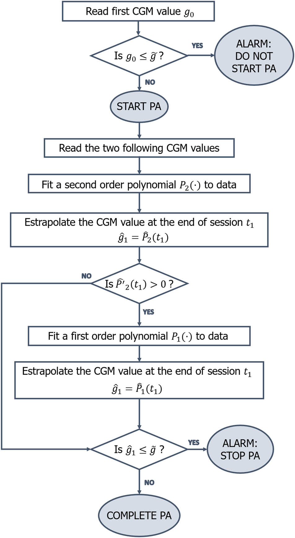
Flowchart of the “Real-time PA” algorithm.
For the “Starting PA” algorithm, we want to estimate for any individual the probability
To find the most suitable shape for the probability density function
Here, the function
The same procedure can also be applied describing the CGM function with a polynomial of degree two
The values of
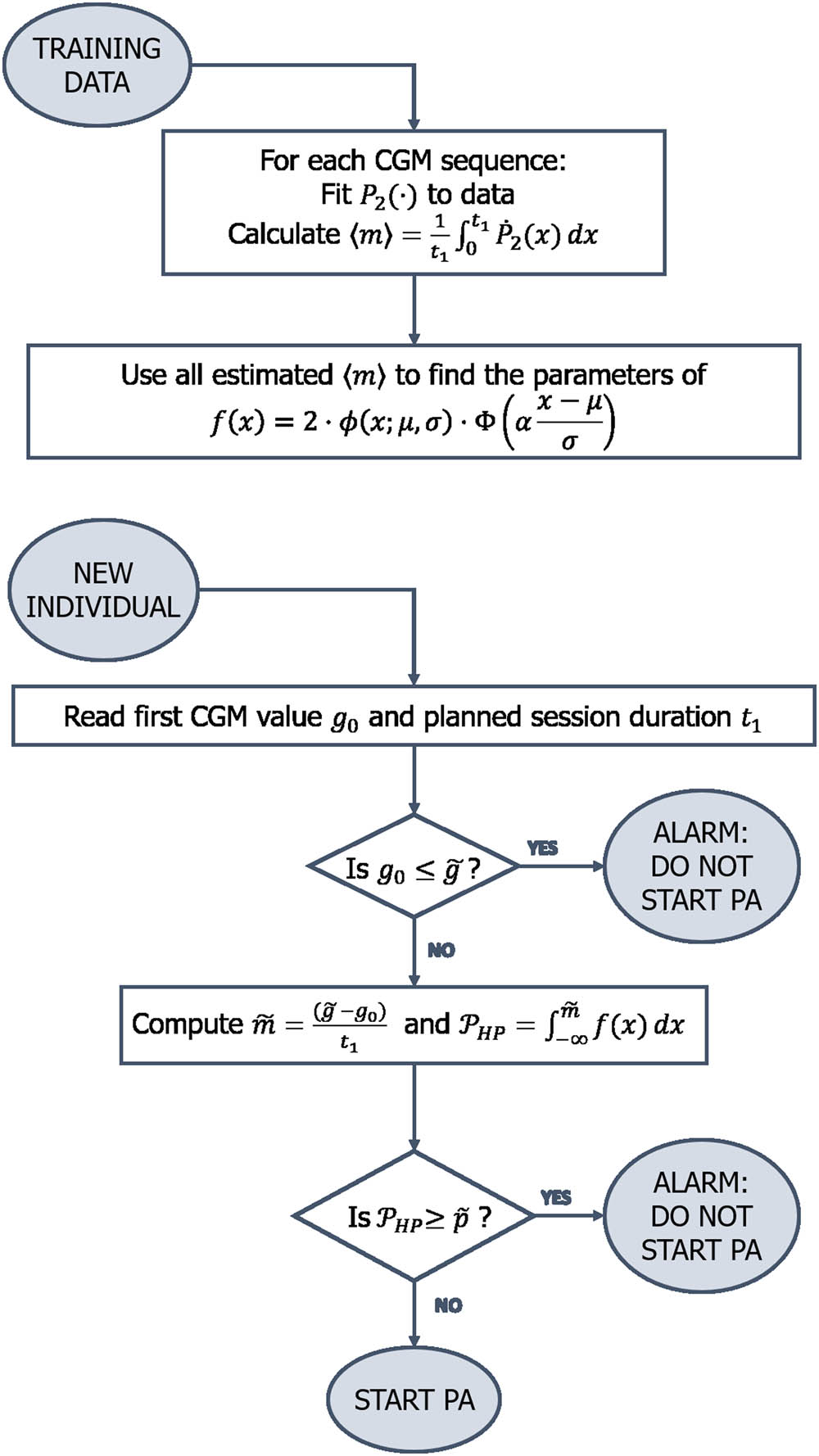
Flowchart of the “Starting PA” algorithm.
2.2 Performance quantification procedures
To evaluate the prediction performance of the two proposed algorithms, we proceed as follows. For the “Real-time PA” algorithm, using the estimated model to extrapolate CGM data, we assess the occurrence of HP in
We turn now to the assessment of the “Starting PA” algorithm. Let us first consider any partition of the whole set of sessions into two disjoint sub-samples of about the same size. One of these subsets is used for training, i.e. to estimate the parameters of the model
In addition to the AUC, we also consider another global performance indicator. Let us consider any partition of the whole set of PA sessions. As commonly done, we introduce the accuracy, defined as the arithmetic average between sensitivity and specificity curves. We notice that empirically this curve presents a global maximum. Therefore, it can be of interest to evaluate sensitivity and specificity curves at the threshold value
where
After performing the described validation study for the “Starting PA” algorithm, when applying it to a new individual, we wish to use the information about the distribution of the average rate of decrease of the CGM theoretical model, as derived from the whole set of considered sessions. The situation closest to it, which still enables us to assess the algorithm performance, is concerned with the leave-one-out cross validation [27]. Following this scheme, we select in turns each of the
Finally, we report some results concerning with sessions for which we properly predict HP. For the “Real-time PA” algorithm, we compute the average of the difference between the time
3 Results
The following results are obtained applying the two methodologies to the data from the T1DEXI study of the Jaeb Center for Health Research [20,21]. The dataset contains several information from 497 people with T1D between 18- and 70-years old performing controlled PA. The majority of the subjects are between 26 and 44 years old (51%), while the 22% is younger than 26 and the remaining 27% older. The database present an imbalance between females and males, with the first group representing the 73% of the whole sample. Almost half of the sample have a hybrid closed-loop system (45%), the 37% adopt a standard insulin pump, while only the 18% uses multiple daily injections. More details can be found in Riddell et al. [20]. In that study, the subjects were divided into three groups of about the same size, and all individuals of each group were assigned to a specific training type between resistance (172 subjects), aerobic (163 subjects) and interval (167 subjects). Each subject performed several PA sessions, recorded in study videos, of variable length with a median value of about 30 min. During each PA session, the glucose concentration in peripheral blood was acquired by CGM device every 5 min.
We now focus on the “Real-time PA” algorithm. To quantify its performance, we select PA sessions, among all those available, according to the following criteria. We require at least three CGM readings in the interval
Inclusion criteria. The three chosen criteria to include a training session in the performance quantification of the “Real-time PA” algorithm
| Number of CGM readings in
|
| Starting CGM value
|
| Average slope of the fit
|
Summarizing, for the “Real-time PA” algorithm, we analyse a total sample of 1,022 sessions, 500 of which resistance (RES), 337 aerobic (AER) and 185 interval (INT). The algorithm is applied the same way to each CGM sequence of the 1,022 sessions, irrespective of the type of training. In Figure 3, we present two examples of the adopted theoretical model fitted to CGM data. In the left (right) panel, we show a linear (non-linear) evolution of CGM data, both well described by the quadratic theoretical model
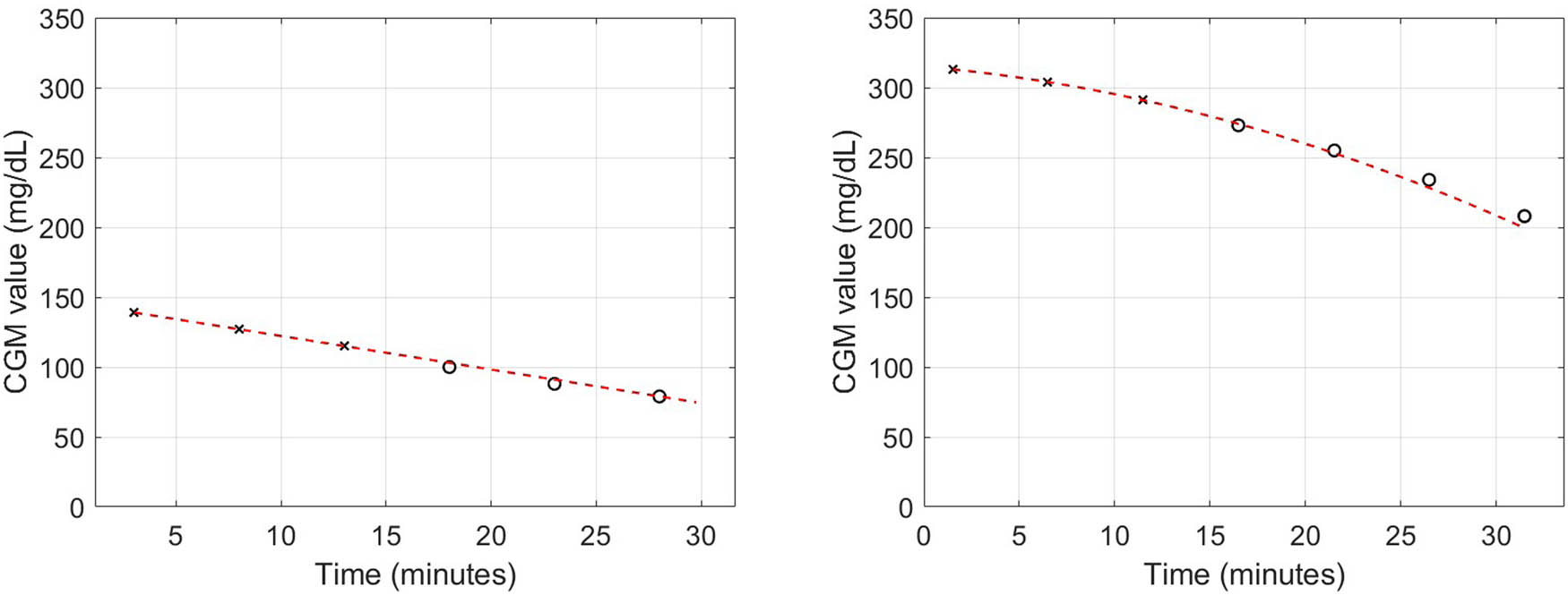
Examples of measured CGM sequence and theoretical model. The theoretical model (dashed line) corresponds to the
Performance results for the proposed “Real-time PA” algorithm applied to the whole set of 1,022 sessions of the three available types
| Indicator | Value | Units |
|---|---|---|
| Sensitivity |
|
% |
| Specificity |
|
% |
| Accuracy | 91 | % |
| RMSE | 12.41 (15.92) | mg/dL |
The percentage value of sensitivity and specificity are reported together with the corresponding absolute numbers of sessions. The sample mean of the RMSE between the CGM data and the theoretical values extrapolated by the model in the prediction interval is also reported together with its standard deviation.
We now turn to the “Starting PA” algorithm. To test its performance, some weaker constraints are imposed to select PA sessions to be analyzed. We notice that the application of this algorithm only needs the value
Summary of some main features of the sessions used for performance quantification of the proposed “Starting PA” algorithm separately for each of the three PA types. In the last two columns, some information about the sessions with HP are also showed
| Type of PA | No. of sessions | Mean
|
No. sessions with HP | % |
|---|---|---|---|---|
| Resistance | 890 |
|
32 | 3.6 |
| Aerobic | 880 |
|
45 | 5.1 |
| Interval | 873 |
|
28 | 3.2 |
| Total | 2,643 |
|
105 | 4.0 |
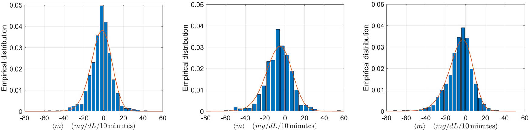
Differently from the “Real-time PA” algorithm, the performance here are evaluated separately for each of the three types of sessions. This choice is motivated by the fact that the empirical distributions of the average rate of decrease of CGM are significantly different for the three types of PA, as shown in Figure 4. However, for completeness, the performances are also quantified by pooling the sessions of the three types. We notice that, to produce the results in the cited figure, for each type of PA, we have used all the sessions available.
The average values of the optimal accuracy, sensitivity and specificity on the same repeated random partitions are reported in Table 4. As already explained, we also perform a leave-one-out cross-validation. The performance obtained from this approach differ in absolute value from those in Table 4 at most of 0.02 for all combinations of indicators and types of training. However, when considering all the sessions together, irrespective of the type of training, the values are identical for each of the four indicators.
Performance indicators for the “Starting PA” algorithm calculated for the three types of sessions
| Type of training | AUC | Sensitivity | Specificity | Accuracy |
|---|---|---|---|---|
| RES | 0.84 (0.76–0.91) | 0.83 (0.69–1.00) | 0.74 (0.66–0.80) | 0.79 (0.72–0.86) |
| AER | 0.85 (0.80–0.89) | 0.83 (0.73–0.94) | 0.68 (0.60–0.75) | 0.77 (0.72–0.82) |
| INT | 0.90 (0.84–0.95) | 0.82 (0.69–1.00) | 0.81 (0.74–0.87) | 0.82 (0.75–0.89) |
| TOT | 0.86 (0.83–0.89) | 0.83 (0.76–0.90) | 0.74 (0.70–0.78) | 0.78 (0.75–0.82) |
The results are obtained from 300 random selections of training and testing sets (50%/50%). The mean values of the indicators are reported together with their 95% quantile intervals.
On the left panel of Figure 5, we display an example of ROC curve for one possible random partition of the whole sample in training and testing set. On the right panel, the corresponding accuracy curve is shown, together with the parametric fit relative to equation (4).
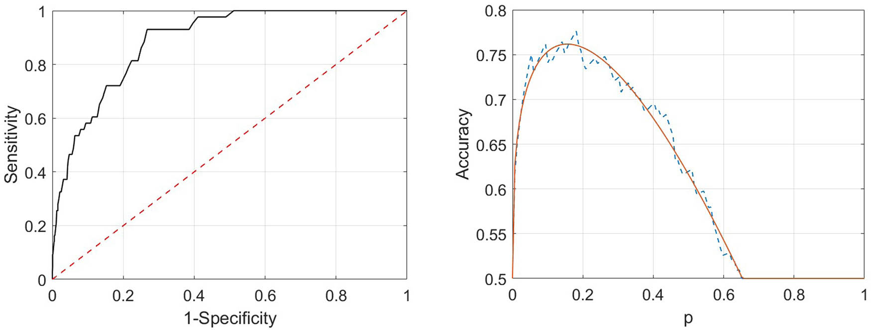
Example of curves of ROC (left panel) and accuracy (right panel) for a possible random choice of training and testing sets (50%/50%). For the accuracy curve, the estimated theoretical model, as in the family in equation (4), is superimposed to the empirical data.
Also in this case, we estimate the length of the forecast interval for predicted HP events and the corresponding starting CGM. The two values are equal to 19.7 min (standard deviation 1) and 93 mg/dL (standard deviation 1.7).
The aforementioned results are relative to the HP threshold level of
We consider now a modification of the method, replacing the quadratic polynomial with a third order one. In fact, the unknown CGM sequence can be fitted here to at least four data points (average data points per PA session 5.6). For each of the three indicators and the different types of training, the performance gain is always below 0.01. This is also true for both the leave-one-out and 50/50 sampling scheme. We note that, for these two variations, we only evaluate the performance for all PA sessions pooled together. In this way, we use the largest sample available and we can assess the influence of these two factors, avoiding to introduce possible effects given by a less accurate estimation procedure.
To possibly improve the performance of the “Starting PA” algorithm by considering other covariates, we proceed as follows. To keep the nice feature of this method, i.e. its simplicity, we only consider the case of a single covariate. Unlike other types of methods, here the covariate identifies sub-samples of sessions with different distributions of the average slope
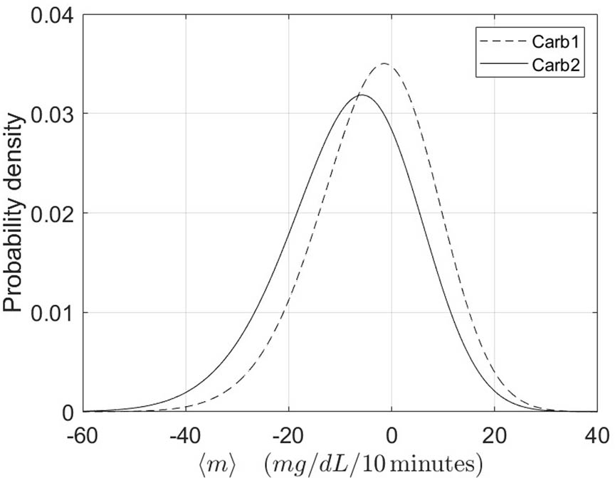
Probability density functions for the two sub-populations of
4 Discussion
The application of the two proposed algorithms to a large database of PA sessions demonstrates their very good ability to predict HP during exercise of people with T1D. Results show higher performance of the “Real-time PA” algorithm when compared to the “Starting PA” one. Anyway, it is interesting to see how, for the “Starting PA” algorithm, sensitivity, which represents the most important indicator for the situation under study, remains larger than
The performance obtained by the “Starting PA” algorithm for INT sessions are, for almost all conditions, higher than the ones obtained from the other two types. This may have two causes, likely related to each other. First, the mean duration of the INT sessions is lower than for the other two types, and consequently, this happens also for the prediction interval. In fact, the INT sessions have a mean duration of 23.7 min (standard deviation 4.4), while RES sessions last in average 31.7 min (standard deviation 3.9), and AER 27.2 min (standard deviation 6.3). Second, measured CGM data for INT sessions are better described by the adopted polynomial function
The overall results show a very good performance of the “Starting PA” algorithm to predict HP. In particular, as mentioned, the sensitivity values remain quite high and stable over the different type of applications (min sensitivity 0.82) and result to be higher than those obtained in Tyler’s [8] (max sensitivity 0.76) and Bergford’s [10] (max sensitivity 0.75) studies. In fact, our methodology outperforms the latter also in terms of AUC (Bergford’s max AUC 0.83) and accuracy level, while presenting accuracy levels comparable to those obtained from Tyler et al. The study of Reddy and colleagues [7] is the one presenting the best results among those presented in the Introduction. Unfortunately, the highest performance values (sensitivity = 0.86, accuracy = 0.87) are reached by the most complex methodology among the two proposed, which includes 10 covariates. The other algorithm is comparable with the “Starting PA” both in terms of number of covariates and of performance results (sensitivity = 0.82, accuracy = 0.80). In order to assess the adequacy of the mathematical model in describing the CGM evolution during PA, we replace the quadratic polynomial by a third order one. However, the gain in performance is very little. Indeed, for each of the three indicators and the different types of training, it remains below 0.01. This is true for both the leave-one-out and for the other type of sampling setup. Regarding the introduction of the adopted covariate, we first notice that it well separates the two sub-populations. In fact, for
Despite its simplicity, the “Real-time PA” algorithm reaches performance higher than all the algorithms present in literature and briefly described in Section 1. In fact, in the best of these studies, Reddy et al. [7] and Bergford et al. [10] obtain values for both sensitivity, specificity and accuracy lower than the “Real-time PA” algorithm, for PA sessions similar to those considered here. This is also true for the results of the study from Tyler and colleagues [8]. As far as it concerns the study of Romero-Ugalde [9], the prediction error, when considering a model training procedure similar to ours, is approximately
Regarding the aforementioned comparison, we recall that, for the “Real-time PA”, we use hypoglycaemic threshold level of
Potential problems or limitations may arise for the application of the proposed algorithms to different sub-populations of T1D subjects and/or to PA characteristics different from those used here. This may involve quantities related to the subject, e.g. age, sex and insulin modality, as well as others related to PA, e.g. intensity and duration. Other factors of the same type of the last ones that may play a role are climate conditions, stress level and activity environment (e.g. outdoor PA). We notice that, for the “Real-time PA” algorithm, all these factors are implicitly take into account, as the prediction is based on the CGM data from an initial part of the PA session. However, for both algorithms, testing of the methods with additional data is needed to quantify the performance in a broader set of conditions. If the amount and variety of data makes it possible, the analysis could be performed separately in groups depending on different types of conditions. Unfortunately, at the moment, we do not have access to such a rich dataset both in terms of size of the sample and in variety of PA conditions. As a general observation, due to the danger of possible events of HP, we think that the use of controlled PA session should be advised in this population.
The methods proposed here have been developed following a classical informative approach. Specifically, we either use a parametric model to describe the glucose function, or we estimate statistical information on glucose rate variation from a sample population and we use it to calculate the probability of hypoglycaemia. Other possible approaches are related to novel machine learning and deep learning methods. The literature on glucose prediction methods from CGM data using such approaches is huge and many significant advances have been made in recent years. Among those, some interesting and effective methods have been developed, which use NN models [11–13]. Li et al. [11] developed a framework based on convolutional NN with the aim of performing personalized prediction of glucose measurements, based on historical CGM data. The method is applied to two clinical datasets and trained on 90 or 10 days of historical data, respectively. Prediction at 30 and 60 min is then performed using a shifting window containing the 16 last previous CGM measurements. In the best case, an RMSE of 19.19 mg/dL is achieved for the 30 min prediction case. De Paoli and colleagues [12] built a jump NN for predicting glucose concentration, specifically trained on subjects who regularly perform PA. The network is trained on at least one day of historical data per subject and the 30 min prediction is then performed using a window of the last 10 previous CGM measurements. Under the best conditions, the RMSE reaches 20.8 mg/dL. A final interesting work is from Allam [13], where a non-linear autoregressive model with exogenous input is integrated with a NN to improve performance for longer prediction horizons. The trained model uses a window of the last 20 previous CGM readings to predict glucose level at a future time ranging from 15 to 100 min. The RMSE for 30 min prediction is 0.91 mmol/L (16.4 mg/dL). We notice that the proposed “Real-time PA” algorithm outperforms all the above methods on the same prediction horizon, in terms of RMSE. Of course, these methods are developed to forecast glucose level in a more general context. Moreover, most of them consider also longer prediction horizons than ours. Nevertheless, despite the good performance and general applicability of such models, they suffer from two drawbacks. First, most of these methods are not specifically designed to detect PA-induced hypoglycaemia. Second, they require a huge amount of data to be trained, which is difficult to obtain in the case we are focusing on. Most important, in all the studies analyzed, the minimum number of CGM readings used as input for the future prediction is 10, whereas here we use only three CGM measurements in the “Real-time PA” algorithm. Therefore, these types of models cannot be applied in our specific context.
The proposed “Real-time PA” algorithm is fully deterministic. Instead, the “Starting PA” is of statistical type. Our future work involves the combination of the two algorithms to produce a Bayesian one. Indeed, when assuming a parametric model for the CGM data, we could combine the data likelihood with an a priori probability on model parameters. The a priori distribution could be estimated based on previous measurements, in line with empirical Bayes approach [28]. This can be applied dynamically as soon as new data are acquired.
We notice that, after the measurement of the CGM data during the initial part of the session, the “Real-time PA” algorithm could be applied dynamically by shifting forward the time intervals where parameter estimation and prediction are performed. We plan to intensively apply and test the two proposed algorithms, possibly improved, as well as the introduced Bayesian one, to new real CGM data from people with T1D performing PA. Indeed, we have just started the acquisition of such data within the EU Horizon 2020 WARIFA project [29] in relation to which this study has been developed. This involves both retrospective and real-time data analysis. Finally, as soon as a sufficiently large number of sessions of the same subject is available, personalization also becomes possible. In fact, the a priori information regarding the average slope can be estimated from such data and then be used when applying the Bayesian method to the data of a new PA session.
The choice of adopting Matlab as framework to implement the developed methodologies has the advantages to combine high numerical precision with user-friendly graphical interface. Moreover, it allows us to produce a stand-alone version of the codes, which have been incorporated in a specific app within the WARIFA project. A subject using the app can easily run one of the two algorithms when performing PA. The system automatically acquires the needed information, i.e. the initial CGM value at the beginning of the session for the “Starting PA” algorithm, or the CGM values in a first part of it for the “Real-time PA” one. Then a visual or audio alarm will be activated, if HP is predicted. This way, the subject can stop the training. A pilot study involving some subjects with T1D within the WARIFA project will allow to test the different functionalities of the current version of the app. When the WARIFA app will be publicly available, subjects with T1D can download and use it as a tool to help them to safely perform PA. The presence of such app can be effective to overcome the fear of subjects with T1D of experiencing HP when performing PA [3–5]. In addition, healthcare providers may also contribute to the spread of the app by encouraging their patients to use it. This way, it could be possible to progressively assess the performances of the algorithms on a large base, eventually contributing to its modifications for improving them.
5 Conclusions
Here, we have proposed two algorithms to predict HP during exercise in individuals with T1D, and we have applied them to a large database of PA sessions. They are only using a few CGM data of the current PA session, which allows them to be widely applied. The performances obtained show a very good ability to predict HP of both the algorithms. Although the “Real-time PA” algorithm slightly outperforms the “Starting PA” one, this last maintains a high sensitivity value. Furthermore, the “Real-time PA,” despite simple, shows better performances than any of those described in the cited literature. When comparing the “Starting PA” with related known methods, it either outperforms them or these last are more complex and involve the use of many covariates, making them applicable in a reduced set of cases. The “Real-time PA” algorithm is fully deterministic, while the “Starting PA” is a statistical one. However, they could be combined to produce a Bayesian one. Once a large amount of data is available for a given individual, personalization of the Bayesian method is also possible. The two methods have been incorporated in a specific app within the WARIFA project [29], which is now going to be tested through a pilot study. The results of this study, which may suggest how to improve the methods, hopefully will make it possible using the app for a large number of people with T1D to perform a planned PA session without experiencing HP.
Acknowledgements
The authors are thankful to the anonymous reviewers for their useful comments and suggestions.
-
Funding information: This project has received funding from the European Union’s Horizon 2020 research and innovation programme under grant agreement No 101017385 (Art. 29.1 GA).
-
Author contributions: All authors accepted the responsibility for the content of the manuscript and consented to its submission, reviewed all the results, and approved the final version of the manuscript. Both authors contributed to the model development, data analysis and manuscript writing. GS conceived the analysis and supervised simulation results. OM performed the implementation and the application of the algorithms.
-
Conflict of interest: Authors state no conflict of interest.
-
Data Acknowledgments: This publication is based on research using data from Jaeb Center for Health Research that has been made available through Vivli, Inc. Vivli has not contributed to or approved, and is not in any way responsible for, the contents of this publication.
-
Data availability statement: Data sharing is not applicable to this article as no new data were created.
References
[1] Maran A, Pavan P, Bonsembiante B, Brugin E, Ermolao A, Avogaro A, et al. Continuous glucose monitoring reveals delayed nocturnal hypoglycaemia after intermittent high-intensity exercise in nontrained patients with type 1 diabetes. Diabetes Tech Therap. 2010;12(10):763–8. 10.1089/dia.2010.0038Search in Google Scholar PubMed
[2] Cockcroft EJ, Narendran P, Andrews RC. Exercise-induced hypoglycaemia in type 1 diabetes. Experiment Physiol. 2020;105(4):590–9. 10.1113/EP088219Search in Google Scholar PubMed
[3] Pinsker JE, Kraus A, Gianferante D, Schoenberg BE, Singh SK, Ortiz H, et al. Techniques for exercise preparation and management in adults with type 1 diabetes. Canad J Diabetes. 2016;40(6):503–8. 10.1016/j.jcjd.2016.04.010Search in Google Scholar PubMed
[4] Colberg SR, Sigal RJ, Yardley JE, Riddell MC, Dunstan DW, Dempsey PC, et al. Physical activity/exercise and diabetes: a position statement of the American diabetes association. Diabetes Care. 2016 Oct;39(11):2065–79. 10.2337/dc16-1728Search in Google Scholar PubMed PubMed Central
[5] Riddell MC, Peters AL. Exercise in adults with type 1 diabetes mellitus. Nature Rev Endocrinol. 2023;19(2):98–111. 10.1038/s41574-022-00756-6Search in Google Scholar PubMed
[6] Zhang L, Yang L, Zhou Z. Data-based modeling for hypoglycaemia prediction: Importance, trends, and implications for clinical practice. Front Public Health. 2023;11:1044059. 10.3389/fpubh.2023.1044059Search in Google Scholar PubMed PubMed Central
[7] Reddy R, Resalat N, Wilson LM, Castle JR, Youssef JE, Jacobs PG. Prediction of hypoglycaemia during aerobic exercise in adults with type 1 diabetes. J Diabetes Sci Tech. 2019;13(5):919–27. 10.1177/1932296818823792Search in Google Scholar PubMed PubMed Central
[8] Tyler NS, Mosquera-Lopez C, Young GM, El Youssef J, Castle JR, Jacobs PG. Quantifying the impact of physical activity on future glucose trends using machine learning. iScience. 2022;25(3):103888. 10.1016/j.isci.2022.103888Search in Google Scholar PubMed PubMed Central
[9] Romero-Ugalde HM, Garnotel M, Doron M, Jallon P, Charpentier G, Franc S, et al. ARX model for interstitial glucose prediction during and after physical activities. Control Eng Practice. 2019;90:321–30. 10.1016/j.conengprac.2019.07.013Search in Google Scholar
[10] Bergford S, Riddell MC, Jacobs PG, Li Z, Gal RL, Clements MA, et al. The type 1 diabetes and exercise initiative: predicting hypoglycaemia risk during exercise for participants with type 1 diabetes using repeated measures random forest. Diabetes Tech Therap. 2023;25(9):602–11. 10.1089/dia.2023.0140Search in Google Scholar PubMed PubMed Central
[11] Li K, Liu C, Zhu T, Herrero P, Georgiou P. GluNet: ADeep learning framework for accurate glucose forecasting. IEEE J Biomed Health Inform. 2020;24(2):414–23. 10.1109/JBHI.2019.2931842Search in Google Scholar PubMed
[12] De Paoli B, D’Antoni F, Merone M, Pieralice S, Piemonte V, Pozzilli P. Blood glucose level forecasting on type-1-diabetes subjects during physical activity: a comparative analysis of different learning techniques. Bioengineering. 2021;8(6):72. 10.3390/bioengineering8060072Search in Google Scholar PubMed PubMed Central
[13] Allam F. Using nonlinear auto-regressive with exogenous input neural network (NNARX) in blood glucose prediction. Bioelectronic Med. 2024;10(1):11. 10.1186/s42234-024-00141-wSearch in Google Scholar PubMed PubMed Central
[14] Breiman L. Classification and regression trees. Routledge; 2017. 10.1201/9781315139470Search in Google Scholar
[15] Breiman L. Random forests. Machine Learn. 2001;45:5–32. 10.1023/A:1010933404324Search in Google Scholar
[16] Friedman JH. Multivariate adaptive regression splines. Ann Statistics. 1991;19(1):1–67. 10.1214/aos/1176347963Search in Google Scholar
[17] Breton MD, Patek SD, Lv D, Schertz E, Robic J, Pinnata J, et al. Continuous glucose monitoring and insulin informed advisory system with automated titration and dosing of insulin reduces glucose variability in type 1 diabetes mellitus. Diabetes Tech Therap. 2018;20(8):531–40. 10.1089/dia.2018.0079Search in Google Scholar PubMed PubMed Central
[18] Akaike H. Fitting autoregressive for prediction models. Statist Math. 1969;21:243–7. 10.1007/BF02532251Search in Google Scholar
[19] Akaike H. Statistical predictor identification. Ann Inst Stat Math. 1970;22(1):203–17. 10.1007/BF02506337Search in Google Scholar
[20] Riddell MC, Li Z, Gal RL, Calhoun P, Jacobs PG, Clements MA, et al. Examining the acute glycemic effects of different types of structured exercise sessions in type 1 diabetes in a real-world setting: the type 1 diabetes and exercise initiative (T1DEXI). Diabetes Care. 2023 Feb;46(4):704–13. 10.2337/dc22-1721Search in Google Scholar PubMed PubMed Central
[21] Type 1 Diabetes EXercise Initiative: The Effect of Exercise on Glycemic Control in Type 1 Diabetes Study; 10.25934/PR00008428.1. Search in Google Scholar
[22] Seaquist ER, Anderson J, Childs B, Cryer P, Dagogo-Jack S, Fish L, et al. Hypoglycemia and diabetes: a report of a workgroup of the American diabetes association and the endocrine society. Diabetes Care. 2013 Apr;36(5):1384–95. 10.2337/dc12-2480Search in Google Scholar PubMed PubMed Central
[23] Hanley JA, McNeil BJ. The meaning and use of the area under a receiver operating characteristic (ROC) curve. Radiology. 1982;143(1):29–36. 10.1148/radiology.143.1.7063747Search in Google Scholar PubMed
[24] Longato E, Vettoretti M, Di Camillo BA practical perspective on the concordance index for the evaluation and selection of prognostic time-to-event models. J Biomed Inform. 2020;108:103496. 10.1016/j.jbi.2020.103496Search in Google Scholar PubMed
[25] Wolbers M, Koller MT, Witteman JC, Steyerberg EW. Prognostic models with competing risks: methods and application to coronary risk prediction. Epidemiology. 2009;20(4):555–61. 10.1097/EDE.0b013e3181a39056Search in Google Scholar PubMed
[26] Carlin BP, Louis TA. Bayesian methods for data analysis. CRC Press; 2008. 10.1201/b14884Search in Google Scholar
[27] Stone M. Cross-validatory choice and assessment of statistical predictions. J R Stat Soc Ser B (Methodological). 2018 Dec;36(2):111–33. 10.1111/j.2517-6161.1974.tb00994.xSearch in Google Scholar
[28] Carlin BP, Louis TA. Bayes and empirical Bayes methods for data analysis. London: Chapman & Hall; 1996. Search in Google Scholar
[29] Watching The Risk Factors: Artificial Intelligence (AI) and The Prevention of Chronic Conditions; https://www.warifa.eu/[Last access: 02/04/2024]. Search in Google Scholar
© 2025 the author(s), published by De Gruyter
This work is licensed under the Creative Commons Attribution 4.0 International License.
Articles in the same Issue
- Research Articles
- Relationship between body mass index and quality of life, use of dietary and physical activity self-management strategies, and mental health in individuals with polycystic ovary syndrome
- Evaluating the challenges and opportunities for diabetes care policy in Nigeria
- Body mass index is associated with subjective workload and REM sleep timing in young healthy adults
- Prediction of hypoglycaemia in subjects with type 1 diabetes during physical activity
- Investigation by the Epworth Sleepiness Scale of daytime sleepiness in professional drivers during work hours
- Understanding public awareness of fall epidemiology in the United States: A national cross-sectional study
- Impact of Covid-19 stress on urban poor in Sylhet Division, Bangladesh: A perception-based assessment
- Impact of the COVID-19 pandemic on mental health, relationship satisfaction, and socioeconomic status: United States
- Psychological factors influencing oocyte donation: A study of Indian donors
- Cervical cancer in eastern Kenya (2018–2020): Impact of awareness and risk perception on screening practices
- Older LGBTQ+ and blockchain in healthcare: A value sensitive design perspective
- Trends and disparities in HPV vaccination among U.S. adolescents, 2018–2023
- Do cell towers help increase vaccine uptake? Evidence from Côte d’Ivoire
- In search of the world’s most popular painkiller: An infodemiological analysis of Google Trend statistics from 2004 to 2023
- Brain fog in chronic pain: A concept analysis of social media postings
- Association between multidimensional poverty intensity and maternal mortality ratio in Madagascar: Analysis of regional disparities
- A “disorder that exacerbates all other crises” or “a word we use to shut you up”? A critical policy analysis of NGOs’ discourses on COVID-19 misinformation
- Smartphone use and stroop performance in a university workforce: A survey-experiment
- Review Articles
- The management of body dysmorphic disorder in adolescents: A systematic literature review
- Navigating challenges and maximizing potential: Handling complications and constraints in minimally invasive surgery
- Examining the scarcity of oncology healthcare providers in cancer management: A case study of the Eastern Cape Province, South Africa
- Dietary strategies for irritable bowel syndrome: A narrative review of effectiveness, emerging dietary trends, and global variability
- The impact of intimate partner violence on victims’ work, health, and wellbeing in OECD countries (2014–2025): A descriptive systematic review
- Nutrition literacy in pregnant women: a systematic review
- Short Communications
- Experience of patients in Germany with the post-COVID-19 vaccination syndrome
- Five linguistic misrepresentations of Huntington’s disease
- Letter to the Editor
- PCOS self-management challenges transcend BMI: A call for equitable support strategies