Analysis of traffic density dynamics under varied noise conditions using data-driven partial differential equations

1 Introduction

In various applied sciences and engineering, partial differential equations (PDEs) are extremely crucial for modeling and solving several complication occurrences in the real world. They provide a powerful framework for describing natural phenomena. Hence, knowledge of traffic flow behavior becomes important for controlling traffic congestion and enhancing the protection of life. The Burger equation

is a useful instrument in accomplishing such a goal. The equation describes some features of traffic behavior, such as the formation of congestion and the diffusion of traffic. Applying it in actual traffic scenarios, including traffic lights and other traffic control features, is inserted into these elements and can provide information about how traffic flow can be maximized or minimized.

Traditionally, deriving governing PDEs required substantial intuition and scientific expertise. To derive the governing PDEs for a certain system. This review explores the recent paradigm shift in PDE discovery, where data-driven methods are transforming our ability to identify the underlying mathematical rules purely from observation. In recent years, there has been a noticeable increase in efforts to derive PDEs directly from data. So, with the integration of deep learning and physical knowledge, governing equations can now be determined directly from observational data. This paradigm shift holds great promise for scientific advancement across a wide range of disciplines, including biology, engineering, physics, and economics. This emerging discipline aims to bridge the gap between experimental observations and fundamental principles, as pioneered by publications such as [1]. Later on, sparse optimization methods are utilized [2] to extract hidden PDEs from data, laying the groundwork for subsequent advancements. Developing deep learning architectures for PDE discovery has brought considerable advancements to this field [1], [2], [3], [4]. Deep learning, a subset of machine learning, can identify nuanced patterns from large volumes of data, enabling the extraction of governing PDEs from complex and potentially noisy datasets. The DL-PDE framework, introduced by Xu et al. [4], efficiently learns the correspondence between physical systems and their related model equation. A significant advantage in practical applications is that this work demonstrated deep learning’s capacity to handle discrete and noisy input, showcasing its robustness and effectiveness.

Subsequent research has improved data-driven discovery methods by building on this foundation. A potent paradigm that integrates physical rules within the deep learning framework is the concept of physics-informed neural networks (PINNs) [5], 6]. This approach incorporates prior scientific knowledge into the learning process, yielding more reliable and interpretable results.

The field of PDE discovery is rapidly evolving as scientists explore new deep learning architectures and apply uncertainty quantification methods to improve the reliability and generalizability of the PDEs they find [7], [8], [9]. For real-world phenomena, a common challenge is handling sparse and noisy data. For this, Stephany and Earls [7] introduced a deep learning framework PDE-LEARN. The robustness of the Physics-Informed Information Criterion (PIC) method in handling noise while discovering PDEs has been particularly notable. The PIC method can robustly identify the correct PDE forms even with high noise levels. For instance, it can handle up to 75 % noise in some cases and is remarkably robust up to 200 % noise in specific examples like the convection–diffusion and Klein–Gordon equations. This robustness is significantly higher than that of many state-of-the-art methods, making PIC particularly effective in practical applications involving noisy data.

The current research will analyze the discovered PDEs using 200,000 discrete data points with different noise levels [3]. The equation with σ = 1 and ν = −0.01 is a true equation. And the equations resulting from noise data are presented in 1 (Table 1).

A key concept in nonlinear research is finding accurate solutions to nonlinear equations. Although many approaches are available for specific classes of differential equations [10], an algebraic method applicable to a broader range of nonlinear equations is precious. One notable application of the Lie symmetry approach is its ability to efficiently reduce, solve, and simplify complex nonlinear differential equations, making them more manageable [11], 12].

Classifying invariant solutions is the focus of this study. To this end, we find the optimal system of one-dimensional Lie subalgebras within the symmetry algebra of the equation. Sorting the problem according to its admitted symmetry algebra simplifies the task of determining all the optimal subalgebras in one dimension and the corresponding invariant solutions. This allows us to group invariant solutions into non-similar classes. A representative element from the optimal system is used to obtain an invariant solution for each class, providing an effective and systematic method to categorize these solutions. This method involves finding the optimal systems of subalgebras within the Lie symmetry algebras, leading to non-similar invariant solutions under symmetry transformations. The construction of the family of invariant solutions is discussed in detail in [13], 14]. Raza [15] gives Lie symmetry analysis along with the optimal system on non-linear wave equation. Moreover, Jhangeer [16] uses the optimal system to reduce the bi-Hamiltonian Boussinesq system.

The concept of a traveling wave solution is vital in many fields of science and engineering, especially for PDE. The waveform in this solution is considered to have constant speed and shape. Jhangeer [17] studied the geophysical Korteweg–de Vries equation through the Lie approach along with the traveling wave. Moon [18] examines the impact of a change of parameter on the traveling wave solution of the Burger equation with variable coefficients. A two-lane cellular automaton traffic model equivalent to the extended Burgers model has been developed, revealing several metastable and synchronized states in traffic flow by Fukui et al. [19]. Liu [20] explores the general Burgers equation of a spatial and a temporal variable via the Lie approach with variable coefficient. Moreover, extended Lie symmetry analysis of the two-dimensional degenerate Burgers equation is studied by Olena [21]. Zeng et al. [22] constructed a multi-value cellular automata model with Lagrange coordinates, which demonstrated that the density of traffic and the number of lanes have a strong impact on flow.

This paper is structured as follows: In Section 2, we computed Lie symmetries, while Section 3 presents the optimal system. Section 4 discusses the computation of traffic flow densities and we explore the propagation of traffic density dynamics under varied noise by using abelian algebra.

2 Lie symmetries

The current section presents the Lie approach for the considered Eq. (1). Now, consider the one-parameter Lie group of infinitesimal transformations given by

The corresponding vector field is

Then it will be the Lie point symmetry generator of Eq. (2) with solutions of Eq. (1) if

where X [ 2 ] is the second prolongation which can determined by

Applying invariance condition to Eq. (1), we have

Where,

where D i is defined as:

By substituting η ⁱ from equation Eq. (4), we obtained the ensuing five-dimensional Lie algebra:

But for the actual true PDE that governs the observed physical process we have,

2.2 Computation of traffic flow densities

In the current section, we will utilize the previously discussed optimal system to reduce equation (1). We can obtain exact solutions for the given equations by symmetry reduction by employing equivalence classes of symmetry generators. This method is a well-defined algorithmic process, which is described in the standard literature on this topic, in particular in textbooks [13], 23]. Group invariant solutions can be easily generalized to PDEs with any number of independent and dependent variables. The number of independent variables can be reduced to one by using a one-parameter group that has nontrivial effects on one or more of the independent variables. So for this, we employ the invariant form approach and explicitly address the invariance surface conditions with the help of solving the characteristic form defined as:

(8) d t τ ( x , y , t , u ) = d x ξ ( x , y , t , u ) = d y γ ( x , y , t , u ) = d u η ( x , y , t , u ) .

We will also derive the traveling wave solution using the traveling wave variable ζ = α − λβ for the reduced PDEs. The traveling wave solution is of the form

w ( α , β ) = f ( ζ ) , ζ = α − λ β ,

When this form is applied to the reduced PDE, corresponding to X 4 , it yields the following traveling wave ODE:

(9) 1 a 1 − a 2 λ f ′ − σ a 1 ( 1 − λ ) f f ′ + ν a 1 2 ( 1 + λ 2 ) f ″ = 0 .

Considering the generator X 5 , where

(10) X 5 = X 1 + a 3 X 3 ,

and applying Eq. (8), we find that the invariant variables are

(11) α = a 3 t − x , β = y , u = w ( α , β ) .

Thus, Eq. (1) simplifies to

(12) a 3 w α + σ w ( w β − w α ) + ν ( w α α + w β β ) = 0 .

With the aid of computational assistance, we obtain

(13) w ( α , β ) = − 2 ν c 2 2 + c 3 2 tanh ( c 2 α + c 3 β + c 1 ) σ ( − c 3 + c 2 ) + a 3 c 2 σ ( − c 3 + c 2 ) ,

or

(14) u ( x , y , t ) = − 2 ν ( c 2 + c 3 ) tanh ( c 2 ( a 3 t − x ) + c 3 y + c 1 ) σ ( − c 3 + c 2 ) + a 3 c 2 σ ( − c 3 + c 2 ) .

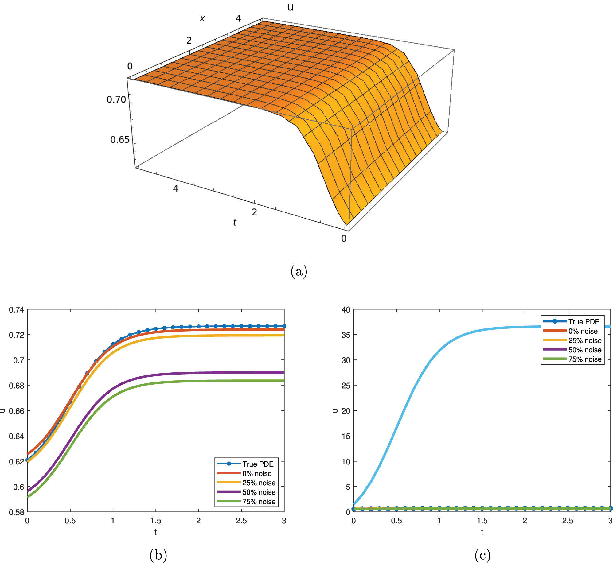
The graphical representation of Eq. (14) is presented in Figure 1. The tanh-type smooth kink solution is obtained, demonstrating how variations in the coefficient scaling the nonlinear advection term and the diffusion coefficient influence traffic flow. Specifically, adjusting these coefficients illustrates the transition from free-flowing to congested traffic, revealing that the system achieves a state with consistent density. When the number of cars entering the route matches the number of vehicles already present, a continuous high-density situation arises, resulting in extremely slow or stop-and-go traffic. Furthermore, the graph of the true PDE, combined with different noise levels identified using a data-driven technique, indicates that the system reaches constant densities at various heights.

Figure 1:

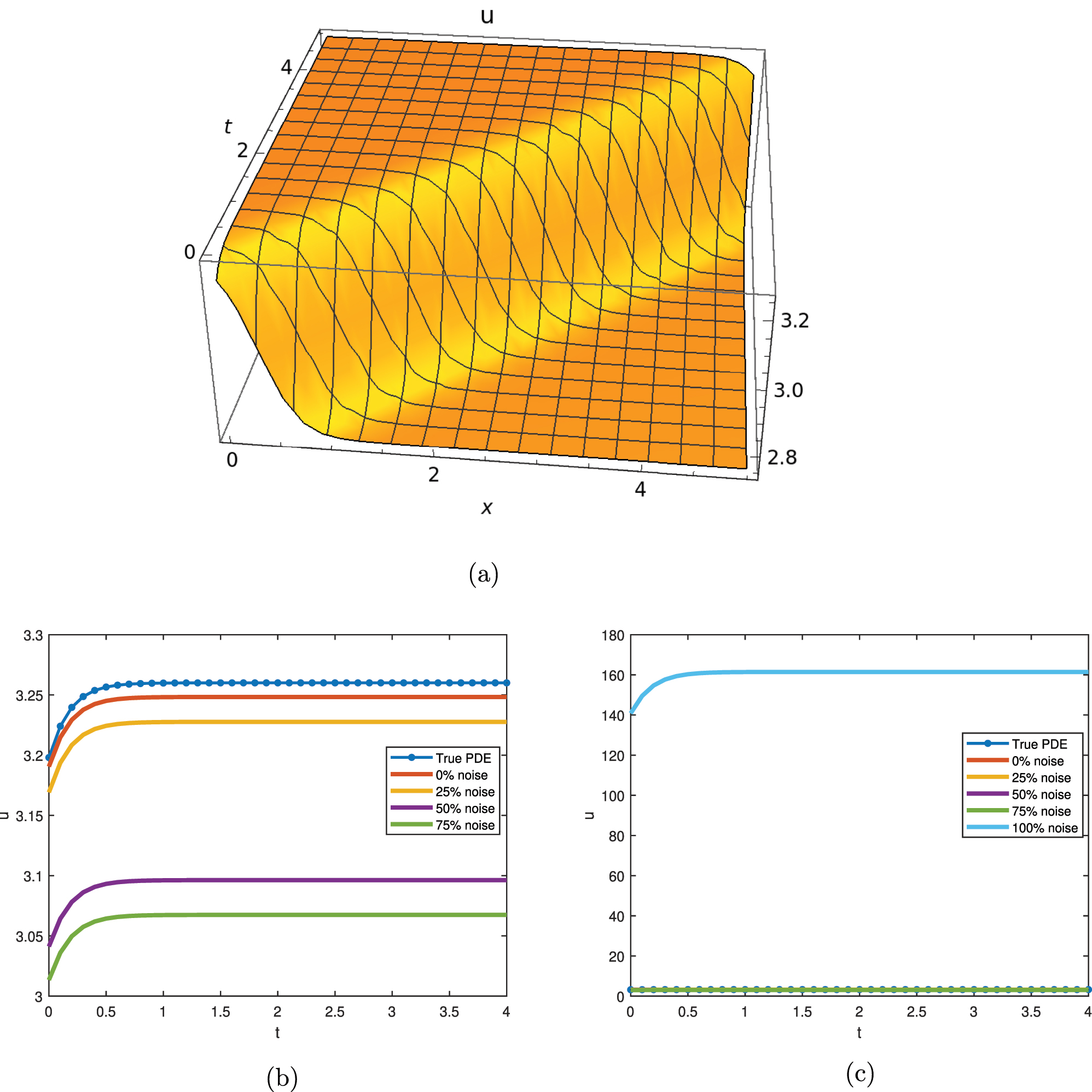
The graphical representation of Eq. (14) with c ₁ = a ₃ = 1, c ₃ = 2, C ₂ = 3. (a) 3D dynamical behavior of traffic flow with ν = −0.01 and σ = 1. (b) 2D dynamical behavior of traffic flow with different noise levels. (c) 2D dynamical behavior of traffic flow with 100 % noise.

Similarly, for PDE reduced by optimal system X 5 , the following traveling wave ODE is obtained:

(15) a 3 f ′ − σ ( 1 + λ ) f f ′ + ν ( 1 + λ 2 ) f ″ = 0 .

The solution becomes:

(16) f ζ = a 3 λ σ + tan 2 c 1 λ 5 ν σ 3 + 6 c 1 λ 4 ν σ 3 + 8 c 1 λ 3 ν σ 3 + 8 c 1 λ 2 ν σ 3 + 6 c 1 λ ν σ 3 + 2 c 1 ν σ 3 c 2 + ζ 2 ν σ λ 3 + λ 2 + λ + 1 σ 2 λ 2 + 2 λ + 1 × 2 c 1 λ 5 ν σ 3 + 6 c 1 λ 4 ν σ 3 + 8 c 1 λ 3 ν σ 3 + 8 c 1 λ 2 ν σ 3 + 6 c 1 λ ν σ 3 + 2 c 1 ν σ 3 + a σ ,

(17) w α , β = a 3 λ σ + tan 2 c 1 λ 5 ν σ 3 + 6 c 1 λ 4 ν σ 3 + 8 c 1 λ 3 ν σ 3 + 8 c 1 λ 2 ν σ 3 + 6 c 1 λ ν σ 3 + 2 c 1 ν σ 3 c 2 + α − λ β 2 ν σ λ 3 + λ 2 + λ + 1 σ 2 λ 2 + 2 λ + 1 × 2 c 1 λ 5 ν σ 3 + 6 c 1 λ 4 ν σ 3 + 8 c 1 λ 3 ν σ 3 + 8 c 1 λ 2 ν σ 3 + 6 c 1 λ ν σ 3 + 2 c 1 ν σ 3 + a σ ,

and

(18) u x , y , t = a 3 λ σ + tan 2 c 1 λ 5 ν σ 3 + 6 c 1 λ 4 ν σ 3 + 8 c 1 λ 3 ν σ 3 + 8 c 1 λ 2 ν σ 3 + 6 c 1 λ ν σ 3 + 2 c 1 ν σ 3 c 2 + a 3 t − x − λ y 2 ν σ λ 3 + λ 2 + λ + 1 σ 2 λ 2 + 2 λ + 1 × 2 c 1 λ 5 ν σ 3 + 6 c 1 λ 4 ν σ 3 + 8 c 1 λ 3 ν σ 3 + 8 c 1 λ 2 ν σ 3 + 6 c 1 λ ν σ 3 + 2 c 1 ν σ 3 + a σ .

The graphical representation of Eq. (18) is shown in Figure 2.

Figure 2:

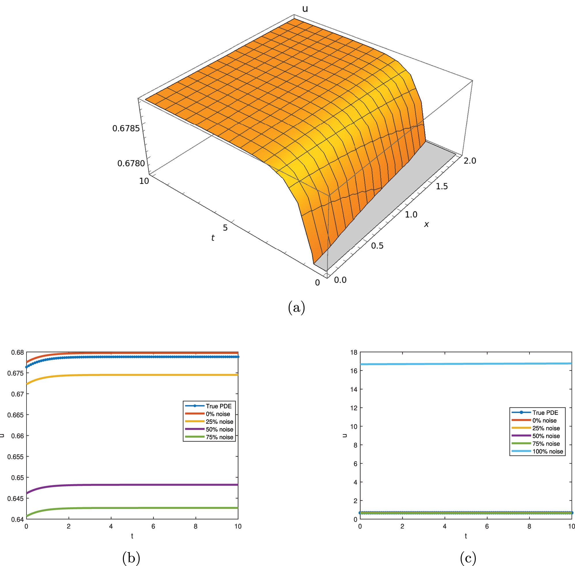
The graphical representation of Eq. (18) with λ = 2, c ₁ = 1/225, c ₃ = 2, a ₃ = 2, C ₂ = 3. (a) 3D dynamical behavior of traffic flow with ν = −0.01 and σ = 1. (b) 2D dynamical behavior of traffic flow with different noise levels. (c) 2D dynamical behavior of traffic flow with 100 % noise.

The graphical outcomes reveal a kink solution with an increasing trajectory in the traffic density profile over the given interval. The curves corresponding to the true PDE, 0 % noise, and 25 % noise levels exhibit similar behavior with less error. However, while the 100 % noise level also shows an increasing trend, it deviates more significantly from the true PDE than other noises.

Similarly, by considering the generator X 6 , viz.

(19) X 6 = X 2 + a 3 X 3 .

The invariant variables are

(20) α = a 3 y − x , β = t , u = w ( α , β ) ,

and the reduced form is

(21) w β + σ ( a 3 − 1 ) w w α + ν 1 + a 3 2 w α α = 0 .

The solution, with computational assistance, is

(22) w ( α , β ) = 2 ⁡ tanh ( c 2 α + c 3 β + c 1 ) ν c 2 ( a 2 + 1 ) σ ( a 3 − 1 ) − c 3 σ c 2 ( a 3 − 1 ) ,

or

(23) u ( x , y , t ) = 2 ⁡ tanh ( c 2 ( a 3 y − x ) + c 3 t + c 1 ) ν c 2 a 3 2 + 1 σ ( a 3 − 1 ) − c 3 σ c 2 ( a 3 − 1 ) .

The graphical representations in Figure 3 demonstrate the impact of different values of coefficients of advection and diffusion on changes across a specified interval. By modifying these coefficients, we note that in up to 75 % of cases, the graphs exhibit behavior that closely resembles previous results, indicating less error. Despite the system eventually reaching a steady state, there is a transition in behavior from free-flowing to congested traffic.

Figure 3:

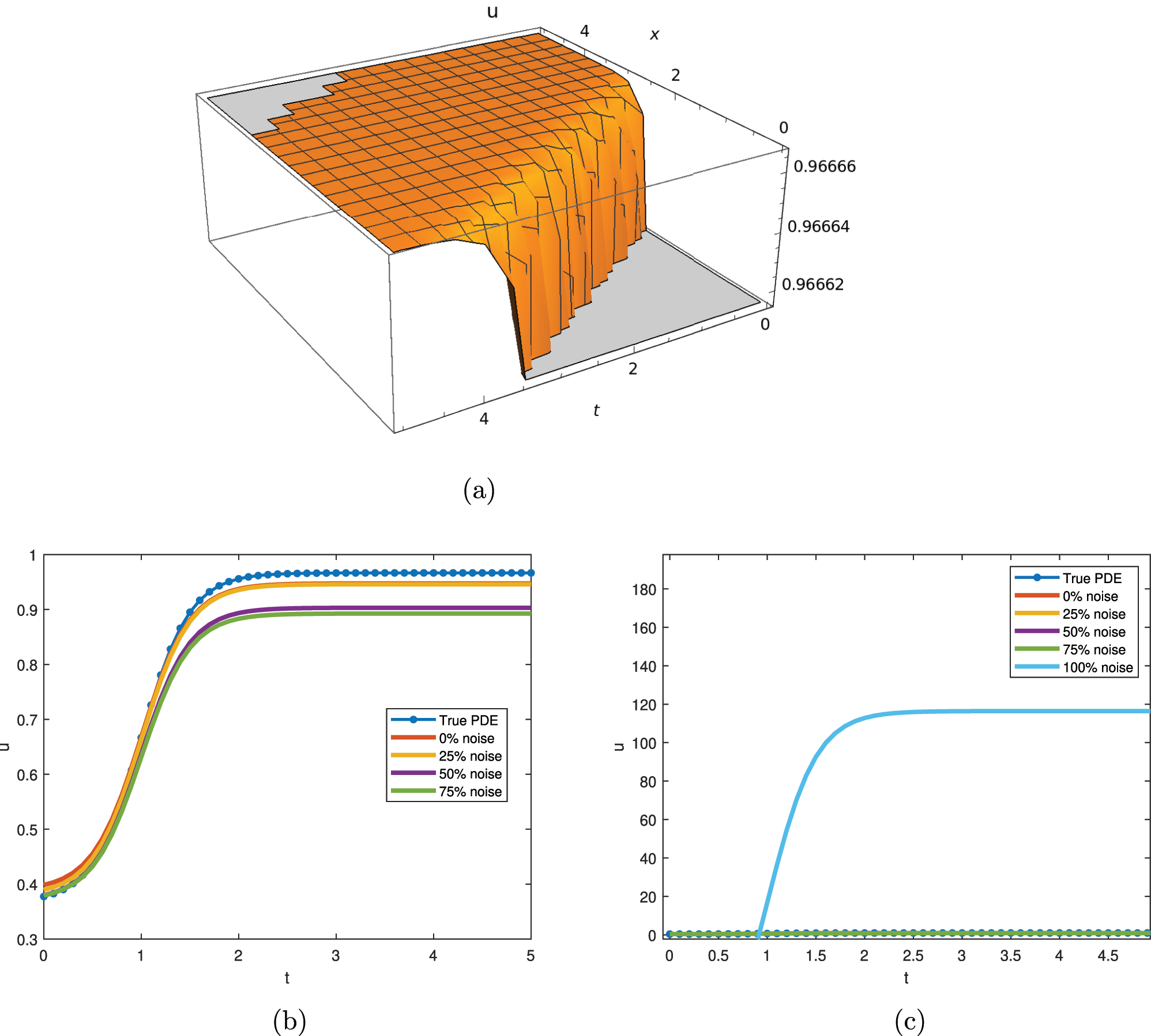
The graphical representation of Eq. (23) with C ₁ = 2, C ₃ = −2, C ₂ = 3, a ₃ = 2. (a) 3D dynamical behavior of traffic flow with ν = −0.01 and σ = 1. (b) 2D dynamical behavior of traffic flow with different noise levels. (c) 2D dynamical behavior of traffic flow with 100 % noise.

For the traveling wave solution represented by the second-order ODE for X 6 , we employ traveling wave variables and obtain

(24) − λ f ′ + σ ( a 3 − 1 ) f f ′ + ν 1 + a 3 2 f ″ = 0 ,

or

(25) f ζ = σ a 3 λ + tanh 2 c 1 a 3 5 ν σ 3 − 6 c 1 a 3 4 ν σ 3 + 8 c 1 a 3 3 ν σ 3 − 8 c 1 a 3 2 ν σ 3 + 6 c 1 a ν σ 3 − 2 c 1 ν σ 3 c 2 + ζ 2 σ ν a 3 3 − a 3 2 + a 3 − 1 σ 2 a 3 2 − 2 a 3 + 1 × 2 c 1 a 3 5 ν σ 3 − 6 c 1 a 3 4 ν σ 3 + 8 c 1 a 3 3 ν σ 3 − 8 c 1 a 3 2 ν σ 3 + 6 c 1 a 3 ν σ 3 − 2 c 1 ν σ 3 − σ λ ,

or

(26) w ( α , β ) = σ a 3 λ + tanh 2 c 1 a 3 5 ν σ 3 − 6 c 1 a 3 4 ν σ 3 + 8 c 1 a 3 3 ν σ 3 − 8 c 1 a 3 2 ν σ 3 + 6 c 1 a ν σ 3 − 2 c 1 ν σ 3 c 2 + α − λ β 2 σ ν a 3 3 − a 3 2 + a 3 − 1 σ 2 a 3 2 − 2 a 3 + 1 × 2 c 1 a 3 5 ν σ 3 − 6 c 1 a 3 4 ν σ 3 + 8 c 1 a 3 3 ν σ 3 − 8 c 1 a 3 2 ν σ 3 + 6 c 1 a 3 ν σ 3 − 2 c 1 ν σ 3 − σ λ ,

or

(27) u ( x , y , t ) = σ a 3 λ + tanh 2 c 1 a 3 5 ν σ 3 − 6 c 1 a 3 4 ν σ 3 + 8 c 1 a 3 3 ν σ 3 − 8 c 1 a 3 2 ν σ 3 + 6 c 1 a ν σ 3 − 2 c 1 ν σ 3 c 2 + a 3 y − x − λ t 2 σ ν a 3 3 − a 3 2 + a 3 − 1 σ 2 a 3 2 − 2 a 3 + 1 × 2 c 1 a 3 5 ν σ 3 − 6 c 1 a 3 4 ν σ 3 + 8 c 1 a 3 3 ν σ 3 − 8 c 1 a 3 2 ν σ 3 + 6 c 1 a 3 ν σ 3 − 2 c 1 ν σ 3 − σ λ .

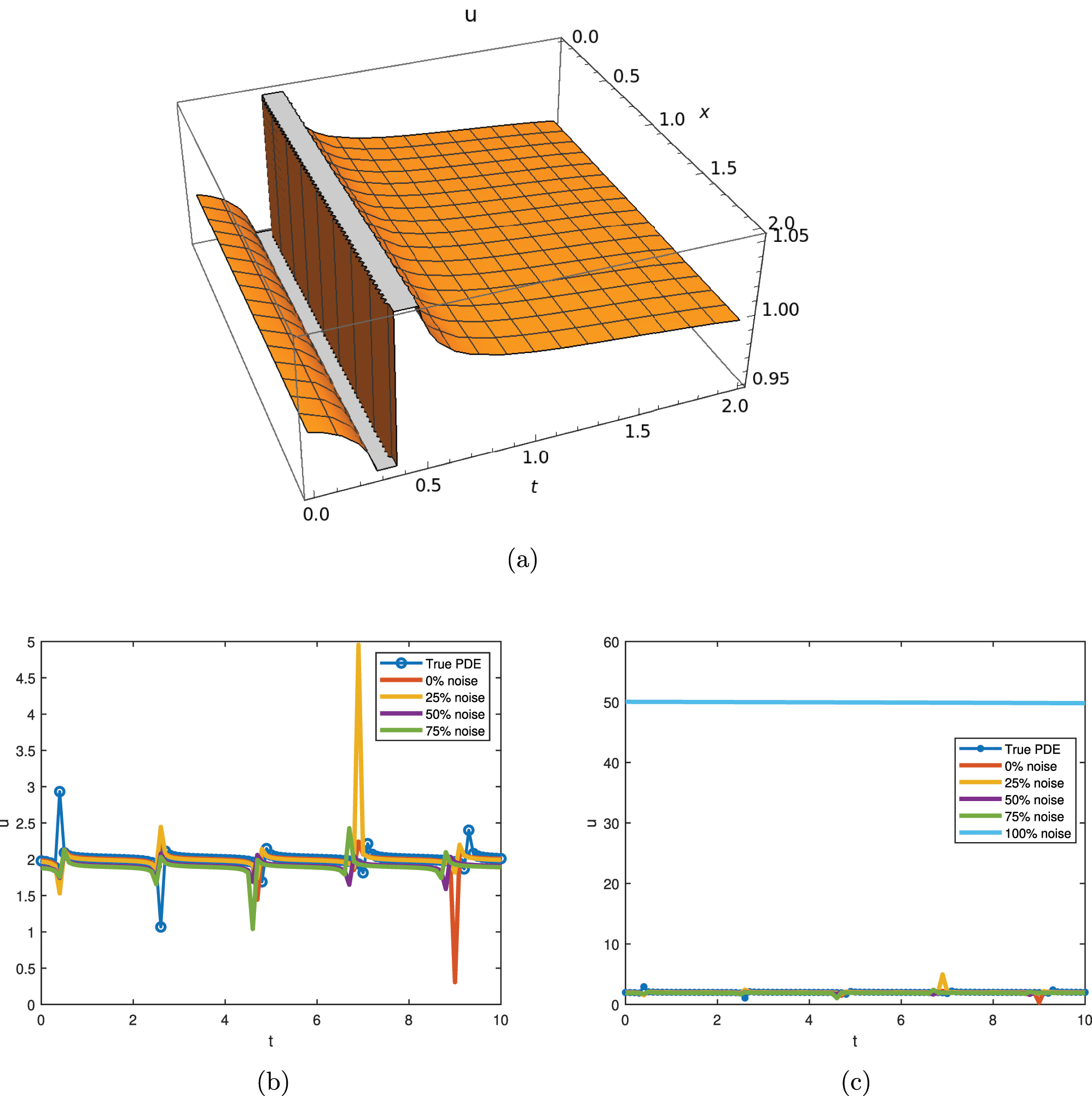
The graphical representation of Eq. (27), is presented in Figure 4. The graphical results represented a singular kink, showing the shock waves in the traffic density graph for all the noise levels and the true PDE. These unexpected results correspond to abrupt changes in traffic conditions, the onset of congestion, or the clearing of a traffic jam. Despite a greater deviation in the curve representing 0 % noise level, it can be observed that the pattern aligns with the true PDE.

Figure 4:

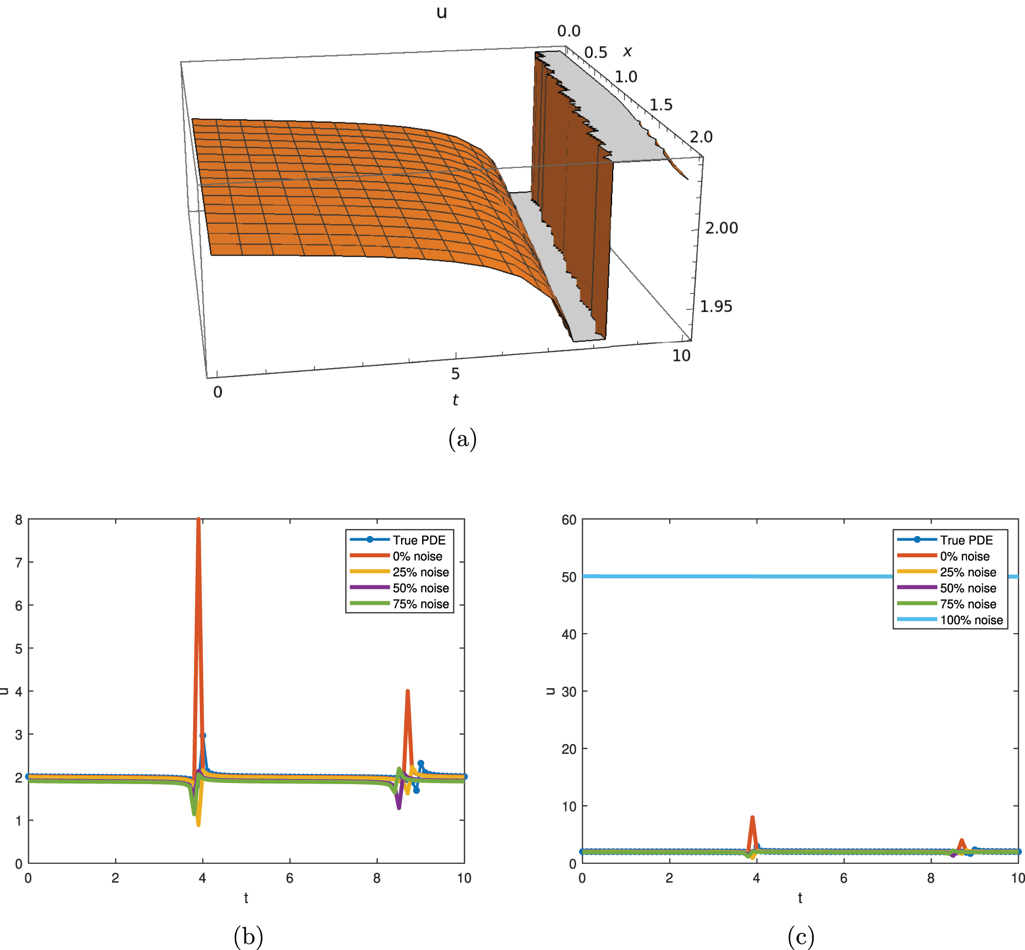
The graphical representation of Eq. (26) λ = 2, C ₁ = 1/1,000, C ₃ = 2, C ₂ = 3, and a ₃ = 2. (a) 3D dynamical behavior of traffic flow with ν = −0.01 and σ = 1. (b) 2D dynamical behavior of traffic flow with different noise levels. (c) 2D dynamical behavior of traffic flow with 100 % noise.

Likewise, for the generator X 7 , we find

(28) α = y , β = t , u = w ( α , β ) ,

as invariant variables, resulting in the reduction of Eq. (1) to

(29) w β + σ w w α + ν w α α = 0 .

Thus, with computational assistance, the solution becomes

(30) w ( α , β ) = 2 c 2 ν ⁡ tanh ( c 2 α + c 3 β + c 1 ) σ − c 3 c 2 σ ,

or

(31) u ( x , y , t ) = 2 c 2 ν ⁡ tanh ( c 2 y + c 3 t + c 1 ) σ − c 3 c 2 σ .

Equation (31) outcomes are represented in Figure 5. It can be observed that the findings are less accurate, but 25 % or less noisy data graphical representations are close to true PDE. However, the results show consistent behavior in transitioning from free-flowing to congested traffic within the observed interval, and once again, a constant state is attained.

Figure 5:

The graphical representation of Eq. (23) with C ₁ = 1, C ₃ = −2, C ₂ = 3, a ₃ = 2. (a) 3D dynamical behavior of traffic flow with ν = −0.01 and σ = 1. (b) 2D dynamical behavior of traffic flow with different noise levels. (c) 2D dynamical behavior of traffic flow with 100 % noise.

Finally, for X 7 , we have the following traveling wave ODE:

(32) − λ f ′ + σ f f ′ + ν f ″ = 0 ,

where

(33) f ( ζ ) = 2 ⁡ tanh c 1 ν σ ( c 2 + ζ ) 2 2 ν c 1 ν σ + 2 λ 2 2 σ ,

or

(34) w ( α , β ) = 2 ⁡ tanh c 1 ν σ ( c 2 + ( α − λ β ) ) 2 2 ν c 1 ν σ + 2 λ 2 2 σ ,

or

(35) u ( x , y , t ) = 2 ⁡ tanh c 1 ν σ ( c 2 + ( y − λ t ) ) 2 2 ν c 1 ν σ + 2 λ 2 2 σ .

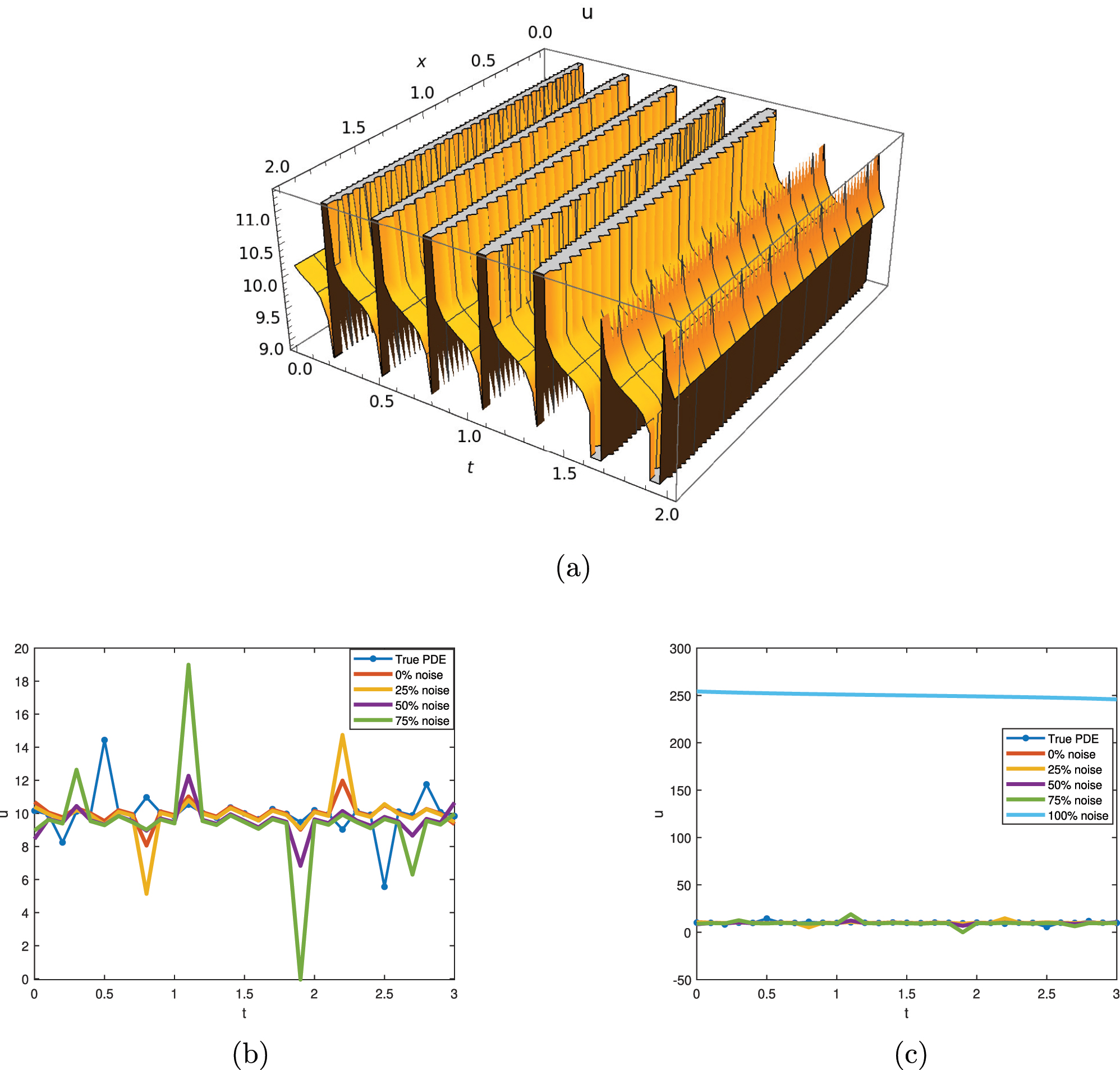
Figure 6 combines three different representations: a 3D visualization of Eq. (35) alongside 2D graphs, illustrating the evolution of traffic flow over time. These graphs show a singular kink solution in the time interval, that shows traffic behavior under sudden changes in conditions such as the unexpected arrival of traffic or the release of a traffic blockage.

Figure 6:

The graphical representation of Eq. (35) with λ = 2, C ₁ = 1/100, C ₃ = 2, C ₂ = 3, and a ₃ = 2. (a) 3D dynamical behavior of traffic flow with ν = −0.01 and σ = 1. (b) 2D dynamical behavior of traffic flow with different noise levels. (c) 2D dynamical behavior of traffic flow with 100 % noise.

Details regarding the reduction by the optimal system are outlined in Table 5.

Table 5:

Reduction by optimal system for Eq. (1).

Generator	α	β	w(α, β)	Reduced PDE
a 1 X 1 + X 4 + X 5	x + σ ( t − a 1 ) a 1 − 2 t	y + σ ( t − a 1 ) a 1 − 2 t	a 1 − 2 t ×	w + αw α  + βw β  + σw(w α  +
			(u + 1)	w β ) + ν(w αα  + w ββ ) = 0
X 1 + X 5	(2t − 1)x −2	x y − 1	xu	2w α  + ν(2w + 10αw α
				−2βw β  + 4α 2 w αα  − 4αβw αβ
				+β 2 w β,β  + 2β 3 w β  + β 4 w ββ ) + σw(−w
				−β 2 w β  − 2αw α  + βw β ) = 0
X 5	tx −2	x y − 1	xu	w α + σ w β w β − w − 2 α w α − β 2 w β
				+ν(2w + 10αw α  − 2βw β  + 4α 2 w αα
				−4αβw αβ  + β 2 w ββ  + 2β 3 w β  + β 4 w ββ ) = 0
a 1 X 1 + a 2 X 2 + X 4	− a 1 x + σ t 2 2	a 2 t + σ t 2 2	− t a 1 + u	1 a 1 + a 2 w β − a 1 σ w ( w α + w β )
		− a 1 y		+ ν a 1 2 ( w α α + w β β ) = 0
X 1 + a 3 X 3	a 3 t − x	y	u	a 3 w α  + σw(w β  − w α )
				+ν(w αα  + w ββ ) = 0
X 2 + a 3 X 3	a 3 y − x	t	u	w β  +
				σ w ( − 1 + a 3 ) w α + ν 1 + a 3 2 w α α = 0
X 3	y	t	u	w β  + σww α  + νw α,α  = 0

2.3 Propagation of traffic density dynamics under varied noise by using abelian algebra

We will now derive the explicit line traveling waves for Eq. (1), by using the traveling wave variable ζ = a x + b y + c t for this derivation. A line-traveling wave in two dimensions is

(36) u ( x , y , t ) = f ( ζ ) , ζ = a x + b y + c t .

By using Eq. (37) in Eq. (1), we obtain a second order ODE

(37) c f ′ + σ ( a + b ) f f ′ + ν ( a 2 + b 2 ) f ″ = 0 .

Then the solution to the ODE is

(38) f ( ζ ) = 1 σ 2 a 2 + 2 a b + b 2 − a c σ − b c σ   + tanh 2 c 1 a 5 ν σ 3 + 6 c 1 a 4 b ν σ 3 + 8 c 1 a 3 b 2 ν σ 3 + 8 c 1 a 2 b 3 ν σ 3 + 6 c 1 a b 4 ν σ 3 + 2 c 1 b 5 ν σ 3 c 2 + ζ 2 ν σ a 3 + a 2 b + a b 2 + b 3 × 2 c 1 a 5 ν σ 3 + 6 c 1 a 4 b ν σ 3 + 8 c 1 a 3 b 2 ν σ 3 + 8 c 1 a 2 b 3 ν σ 3 + 6 c 1 a b 4 ν σ 3 + 2 c 1 b 5 ν σ 3 ,

or

(39) u ( x , y , t ) = 1 σ 2 a 2 + 2 a b + b 2 − a c σ − b c σ + tanh 2 c 1 a 5 ν σ 3 + 6 c 1 a 4 b ν σ 3 + 8 c 1 a 3 b 2 ν σ 3 + 8 c 1 a 2 b 3 ν σ 3 + 6 c 1 a b 4 ν σ 3 + 2 c 1 b 5 ν σ 3 c 2 + a x + b y + c t 2 ν σ a 3 + a 2 b + a b 2 + b 3 × 2 c 1 a 5 ν σ 3 + 6 c 1 a 4 b ν σ 3 + 8 c 1 a 3 b 2 ν σ 3 + 8 c 1 a 2 b 3 ν σ 3 + 6 c 1 a b 4 ν σ 3 + 2 c 1 b 5 ν σ 3 .

The graphical representation of the traveling wave is the singular kink solution represented by Figure 7 with parameters a = 1, b = 2, and c = −2. The fluctuating behavior is an abrupt change in traffic flow density. The graphical comparison between the noise level and the true PDE can also be observed, where more noise results in more derivation. The outcome demonstrates sudden disruptions that larger noise levels result in larger fluctuations.

Figure 7:

The graphical representation of Eq. (39) with c1 = 1 = a, c3 = 2 = b, c = −2 and C2 = 3. (a) 3D dynamical behavior of traffic flow with ν = −0.01 and σ = 1. (b) 2D dynamical behavior of traffic flow with different noise levels. (c) 2D dynamical behavior of traffic flow with 100 % noise.

3 Conclusions

This research analyzed a traffic flow model, which is pivotal for effective traffic management and planning. We investigated the nonlinear model known as the Burger equation through Lie symmetry analysis while varying convection and diffusion coefficients to examine the traffic density curve under different noise levels using traffic data. We established an optimal system and observed that using these optimal systems, as well as the traveling wave solution, yielded various behaviors. Some curves depicted smooth traffic density and the transition from free-flowing to congested traffic. Others exhibited singular kink solutions, indicative of shock waves corresponding to local traffic congestion peaks. By fitting data and adjusting model parameters, specific models for practical problems can be developed. We observed that noise levels of 0 % and 25 % provide the best approximation of the true PDE in smooth patterns. Moreover, understanding these singular kink waves in the traffic density graph is crucial for traffic management and modeling, as they can be influenced by factors such as fluctuating traffic demand, road conditions, and external disturbances.

4 Future directions

The model will be built on in future work to represent the multi-lane traffic dynamics, variable driver behavior and stochastic vehicle arrivals to reflect the reality of traffic conditions. Also, there will be the addition of spatially varying parameters in the effort to represent the heterogeneity of roads and traffic environments. Detailed sensitivity and error analysis will also be used to examine the implications of the PIC in order to examine model robustness when faced with uncertainty. In addition, the proposed framework will be validated over real traffic data in future research, the computational efficiency of large networks will be optimized, and more complex methods based on learning or hybrid methods will be utilized to enhance predictive accuracy and flexibility in dynamic traffic conditions.

References

1. Bongard, J, Lipson, H. Automated reverse engineering of nonlinear dynamical systems. Proc Natl Acad Sci USA 2007;104:9943–8. https://doi.org/10.1073/pnas.0609476104.Search in Google Scholar PubMed PubMed Central
2. Schaeffer, H. Learning partial differential equations via data discovery and sparse optimization. Proc R Soc A 2017;473:20160446. https://doi.org/10.1098/rspa.2016.0446.Search in Google Scholar PubMed PubMed Central
3. Xu, H, Zeng, J, Zhang, D. Discovery of partial differential equations from highly noisy and sparse data with physics-informed information criterion. Research 2023;6:0147. https://doi.org/10.34133/research.0147.Search in Google Scholar PubMed PubMed Central
4. Xu, H, Chang, H, Zhang, D. DL-PDE: deep-learning based data-driven discovery of partial differential equations from discrete and noisy data. arXiv:1908.04463. 2019.Search in Google Scholar
5. Raissi, M. Deep hidden physics models: deep learning of nonlinear partial differential equations. J Mach Learn Res 2018;19:1–24.Search in Google Scholar
6. Raissi, M, Perdikaris, P, Karniadakis, GE. Physics-informed neural networks: a deep learning framework for solving forward and inverse problems involving nonlinear partial differential equations. J Comput Phys 2019;378:686–707. https://doi.org/10.1016/j.jcp.2018.10.045.Search in Google Scholar
7. Stephany, R, Earls, C. PDE-LEARN: using deep learning to discover partial differential equations from noisy, limited data. Neural Network 2024;174:106242. https://doi.org/10.1016/j.neunet.2024.106242.Search in Google Scholar PubMed
8. Zhang, Z, Liu, Y. Robust data-driven discovery of partial differential equations under uncertainties. arXiv:2004.01902. 2020.Search in Google Scholar
9. Xu, H, Zhang, D, Zeng, J. Deep-learning of parametric partial differential equations from sparse and noisy data. Phys Fluids 2021;33:037132. https://doi.org/10.1063/5.0042868.Search in Google Scholar
10. Pelinovsky, DE, Stepanyants, YA. Convergence of Petviashvili’s iteration method for numerical approximation of stationary solutions of nonlinear wave equations. SIAM J Numer Anal 2005;42:1110–27. https://doi.org/10.1137/s0036142902414232.Search in Google Scholar
11. Hydon, P. Symmetry methods for differential equations. Cambridge: Cambridge University Press; 2000.10.1017/CBO9780511623967Search in Google Scholar
12. Ibragimov, NH. Selected works. Karlskrona, Sweden: ALGA Publications; 2006, vol 2.Search in Google Scholar
13. Olver, PJ. Application of lie groups to differential equations. New York, NY, USA: Springer; 1986.10.1007/978-1-4684-0274-2Search in Google Scholar
14. Ovsiannikov, LV. Group analysis of differential equations. New York, NY, USA: Academic Press; 1982.10.1016/B978-0-12-531680-4.50012-5Search in Google Scholar
15. Raza, A, Mahomed, FM, Zaman, FD, Kara, AH. Optimal system and classification of invariant solutions of nonlinear class of wave equations and their conservation laws. J Math Anal Appl 2022;505:125615. https://doi.org/10.1016/j.jmaa.2021.125615.Search in Google Scholar
16. Jhangeer, A. Reduction of non-variational bi-Hamiltonian system of shallow-water waves propagation via symmetry approach. J Math Sci Model 2018;1:39–44. https://doi.org/10.33187/jmsm.411423.Search in Google Scholar
17. Jhangeer, A, Jamal, T, Hussain, MZ, Imran, M. A lie symmetry approach to travelling wave solutions, bifurcation, chaos and sensitivity analysis of the geophysical Korteweg–de Vries equation. Partial Differ Equ Appl Math 2024;10:100734. https://doi.org/10.1016/j.padiff.2024.100734.Search in Google Scholar
18. Moon, B. Traveling wave solutions to the Burgers-αβ equations. Adv Nonlinear Stud 2016;16:147–57. https://doi.org/10.1515/ans-2015-5001.Search in Google Scholar
19. Fukui, M, Nishinari, K, Takahashi, D, Ishibashi, Y. Metastable flows in a two-lane traffic model equivalent to extended Burgers cellular automaton. Physica A 2002;303:226–38. https://doi.org/10.1016/s0378-4371(01)00481-2.Search in Google Scholar
20. Liu, H, Li, J, Zhang, Q. Lie symmetry analysis and exact explicit solutions for general Burgers’ equation. J Comput Appl Math 2009;228:1–9. https://doi.org/10.1016/j.cam.2008.06.009.Search in Google Scholar
21. Vaneeva, OO, Popovych, RO, Sophocleous, C. Extended symmetry analysis of two-dimensional degenerate Burgers equation. J Geom Phys 2021;169:104336. https://doi.org/10.1016/j.geomphys.2021.104336.Search in Google Scholar
22. Zeng, J, Qian, Y, Yin, F, Zhu, L, Xu, D. A multi-value cellular automata model for multi-lane traffic flow under Lagrange coordinate. Comput Math Organ Theor 2022;28:178–92. https://doi.org/10.1007/s10588-021-09345-w.Search in Google Scholar
23. Bluman, G, Anco, S. Symmetry and integration methods for differential equations. Berlin, Germany: Springer Science and Business Media; 2002, vol 154.Search in Google Scholar
© 2026 the author(s), published by De Gruyter, Berlin/Boston
This work is licensed under the Creative Commons Attribution 4.0 International License.
Articles in the same Issue
- Research Articles
- The dynamics of prey–predator model with global warming on carrying capacity and wind flow on predation