Soliton, stability, multistability, and diverse tools for identifying chaos in a nonlinear model with two modified methods
-
Tarmizi Usman
 ,
Noor Alam
,
Noor Alam
 ,
Miguel Vivas-Cortez
,
Muhammad Abbas
,
Miguel Vivas-Cortez
,
Muhammad Abbas

Abstract
This research employs two analytical techniques, the modified Kudrynshov and the modified alternative
1 Introduction
Solitons are distinct waves that do not dissipate or disperse their energy as they propagate through a system [1], 2]. They keep their amplitude and shape as they move through it. These fascinating phenomena arise from the delicate interaction between nonlinearity and dispersion. Many investigators have studied and seen them in various fields, like fluid science, optical fibers, and plasma physics [3], [4], [5], [6]. Accordingly, soliton solutions are quite appealing in nonlinear dynamics [7], [8], [9]. The Z model [10], the Hirota-Maccari framework [11], the generalized KP nonlinear problem [12], the fractional KFG model [13], and other well-known nonlinear models [14], 15] all show that these soliton outcomes are possible. To solve these systems, different techniques exist and provide soliton outcomes. These techniques enclose the expansion method with the
There are many ways to get accurate soliton solutions in the literature. These include the unified solver procedure [34], the extended F-expansion process [35], the new Jacobian elliptic function scheme [36], and the improved modified extended tanh-function [37].
The remaining investigation is outlined below: The graphical abstract is included in Figure 1. Section 2 includes the description of the employed analytical processes, the modified alternative
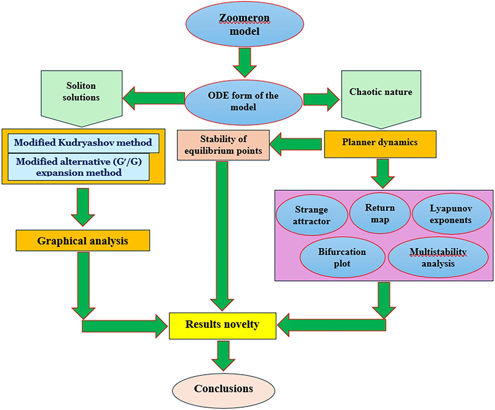
Graphical abstract.
To the best of the author’s knowledge, the modified alternative
2 Analytical methods
Step 1: Consider the following nonlinear system
with the polynomial Ω of the wave function
Step 2: Assume the next linear transformation
where μ and l provide velocity and number of waves, respectively. Using Eq. (2) in Eq. (3), we obtain the subsequent ordinary differential structure of
2.1 Modified alternative
G
′
G
-expansion algorithm
Step 3: Consider the soliton outcome of Eq. (1) with its generalized Riccati equation, which can be written in the form [19]
The relation is obtained from Eq. (5) as
Family 1: When 4LN − M 2 > 0 and MN ≠ 0 (or LN ≠ 0)
where A, B ≠ 0 correspond to the relation A 2 − B 2 > 0.
Family 2: When 4LN − M 2 < 0 and MN ≠ 0 (or N ≠ 0)
where A 2 − B 2 < 0 with A, B ≠ 0.
Family 3: When L = 0 and MN ≠ 0
for the free parameter d.
Family 4: For N ≠ 0 and L = M = 0 (or N ≠ 0)
with an arbitrary constant E.
Step 4: A balancing technique is applied to obtain the value of K described in Eq. (4), which expresses the delicate balance between the highest-order derivatives with the highest degrees of the nonlinear term for Eq. (3).
Step 5: The result obtained by putting the value of K in Eq. (4) with Eq. (3) and Eq. (5), we get a polynomial of
Step 6: Solving the system of algebraic equations obtained in Step 5 gives the initial parameter values of Eq. (3).
2.2 Modified Kudryashov method
Step 3: The initial hypothesis with the ancillary equation of Eq. (1) is written as [24], 25]
with scalars a ≠ 1. The relation is found in Eq. (7) as
with a real number L.
Step 4: A balancing technique is applied to obtain the value of K described in Eq. (6), which expresses the delicate balance between the highest-order derivatives with the highest degrees of the nonlinear term for Eq. (3).
Step 5: The result obtained by putting the value of K in Eq. (6) with Eq. (3) and Eq. (7), we get a polynomial of
Step 6: Solving the system of algebraic equations obtained in Step 5 gives the initial parameter values of Eq. (3).
3 Soliton solutions of the Zoomeron model
The (2 + 1)-D Z model takes the following structure:
Here, the magnitude of the wave is represented by
Here, the integration constant is denoted as q, and the prime notation signifies differentiation with respect to the variable ϑ.
3.1 Applications of the modified alternative
G
′
G
-expansion algorithm to the Z model
Taking K = 1, when X 3 and X″ are balanced. Subsequently, we have the next truncated sequences as
Now, insert Eq. (11) in Eq. (10) and take the coefficient of G i , i = −1, 0, 1 to zero, then the subsequent results are obtained
Now, Eqs. (11) and (12) with the transformation
When
where A, B ≠ 0 correspond to the relation A
2 − B
2 > 0 and ϑ = x + ly − μt with
where ϑ = x + ly − μt with
When
where A, B ≠ 0 correspond to the relation A
2 − B
2 < 0 and ϑ = x + ly − μt with
where ϑ = x + ly − μ with
Here Eqs. (11) and (13) with the transformation
When
where ϑ = x + ly − μt
When
where A, B ≠ 0 correspond to the relation A
2 − B
2 < 0 and ϑ = x + ly − μt
When
with an arbitrary constant d and ϑ = x + ly − μt
When
with an arbitrary constant E and ϑ = x + ly − μt
3.2 Applications of the modified Kudryashov method to the Z model
For K = 1, when X 3 and X″ are balanced. Subsequently, the primary hypothesis Eq. (6) is written as
By plugging Eqs. (7) and (14) into Eq. (10), then take the coefficients of G 0, G, G 2, and G 3 to 0, we get
Now, taking Eqs. (14) and (15) with the transformation
where ϑ = x + ly − μt
4 Figure analysis
The described methods generate various wave solitons in distinct patterns, including kink and anti-kink shapes, bright solitons, localized waves, singular breathers, and multiple breathers.
For y = 0, L = 1, M = 0, μ = 2, A
1 = 1, and q = 6, the curve of
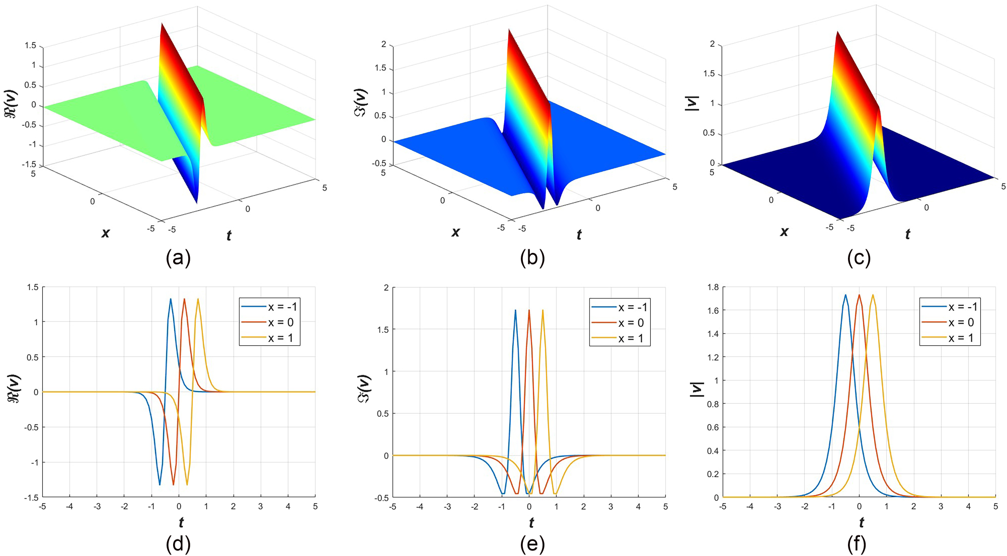
These six patterns represent the profile of v 15 for L = 1, M = 0, μ = 2, A 1 = 1, q = 6. The above (a–c) curves depict 3D and (d–f) curves indicate 2D plots.
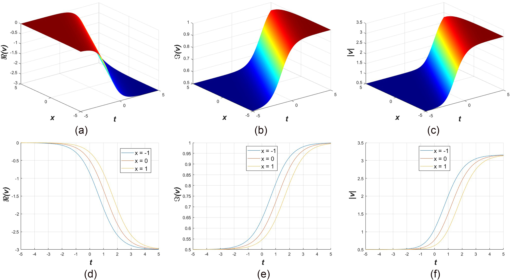
These six formations represent the profile of v 42 for L = 5, μ = 2, q = 1, a = 2. The above (a–c) curves depict the 3D, and (d–f) curves indicate 2D plots.
Furthermore, A breather wave with a singularity can be found in Figure 4(a–c) for the outcome V 14 for q = 1, y = 0, L = 1, M = 0, μ = 2, A 1 = 1. Lastly, in Figure 5(a–c), V 7 indicates multiple bright-dark breather waves for y = 0, L = 1, M = 0, μ = 2, A 1 = 1, q = −1.
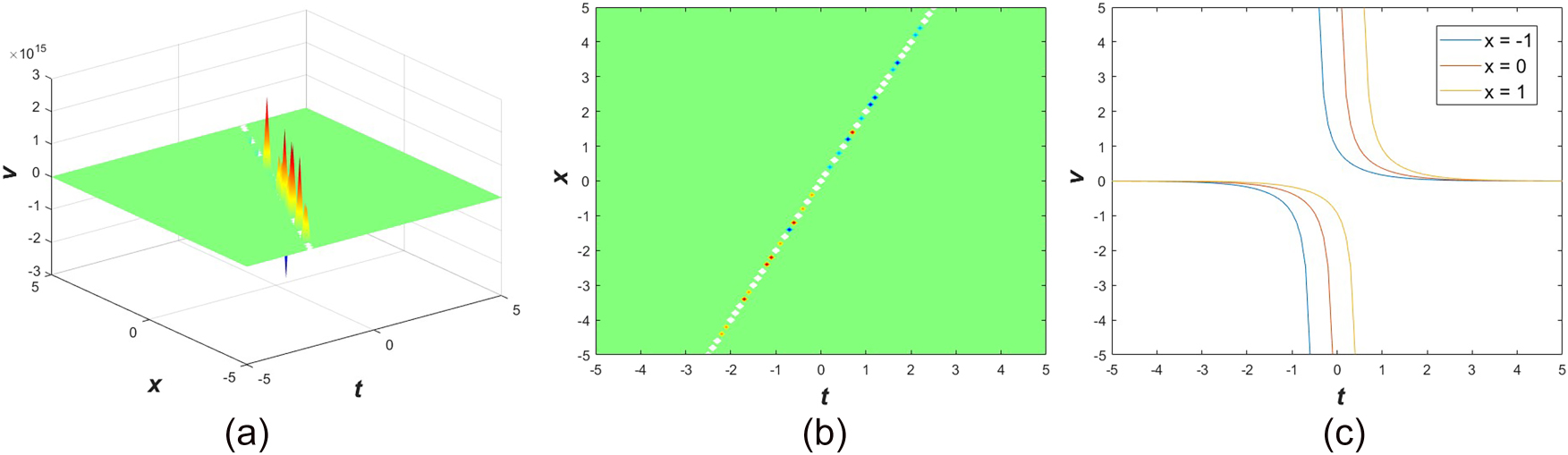
These three views (a–c) represent the profile of v 14 for L = 1, M = 0, μ = 2, A 1 = 1, q = 1. (a) Represents 3D view, (b) depicts density view, and (c) indicates 2D plot.

These three forms represent the profile of v 7 for L = 1, M = 0, μ = 2, A 1 = 1, q = −1. The above (a) depicts the 3D plot, (b) indicates density plot, and (c) indicates 2D plot.
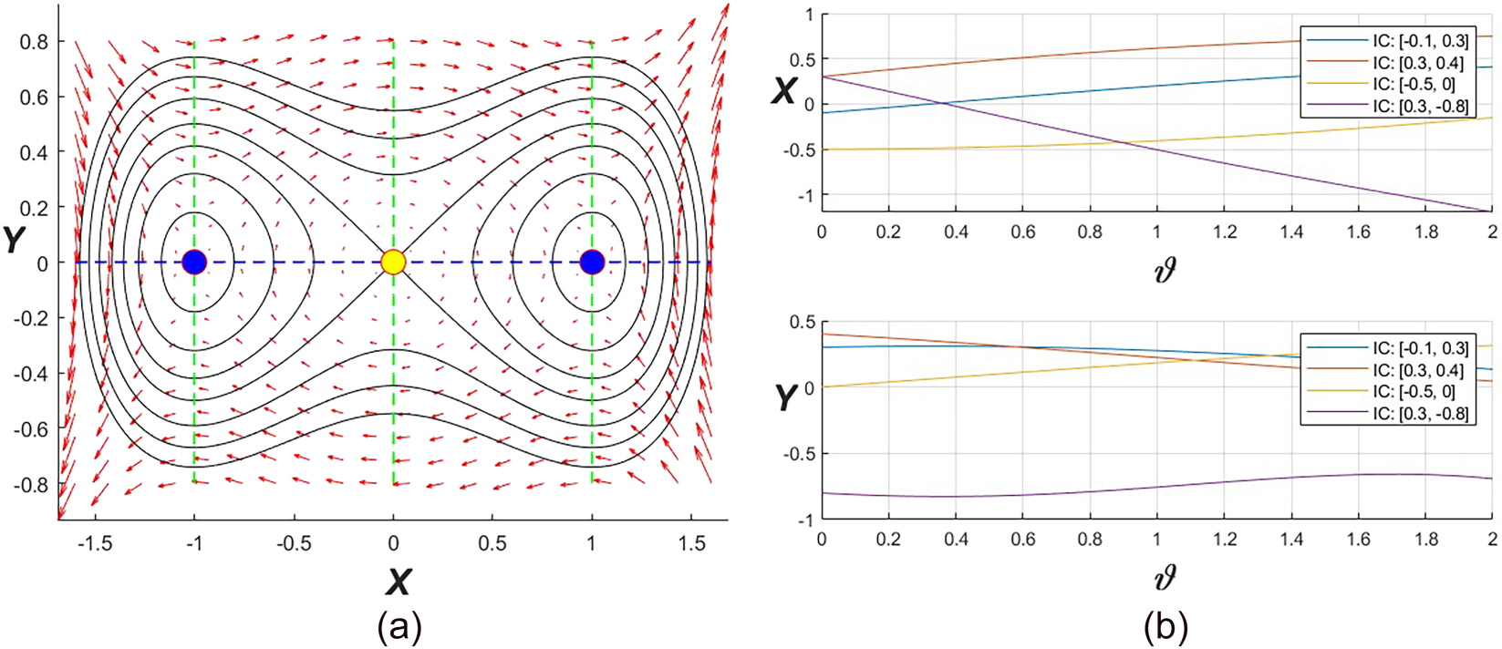
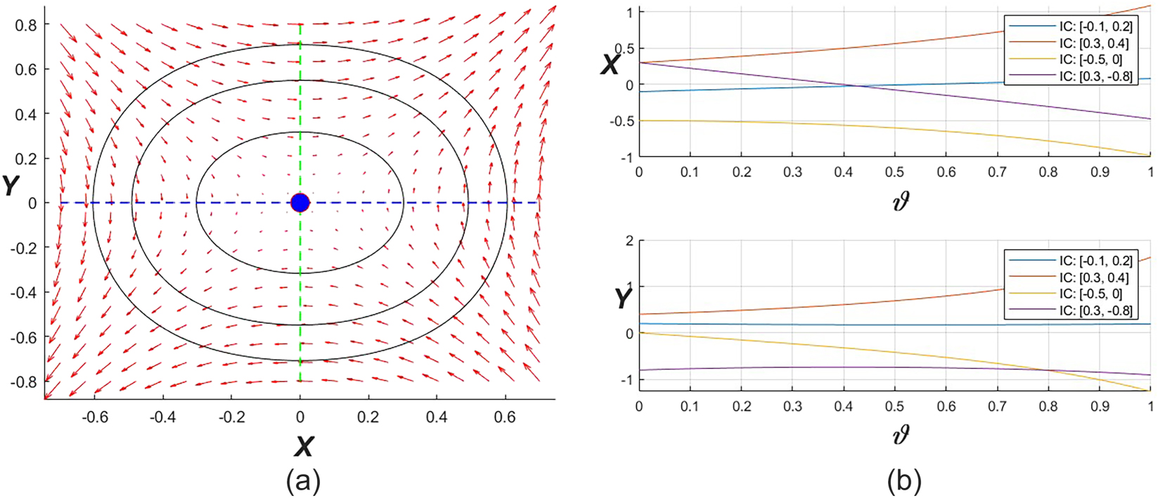
5 Stability analysis for the equilibrium points
For the suggested equation, assume that X′ = Y to explain the phase plane. The alternative form of Eq. (10) in a first-order differential system can be described as follows [39]:
which is the phase plan for the optical outcomes of the Zoomeron model. Equation (10) or (16) derives from the Hamiltonian equation
by consuming the Hamilton canonical form
For q = 0, Eq. (16) gives an equilibrium state as
We know that the Jacobian expression is
The characteristic equation of J corresponds to
Instance 1: Stability at
For

Phase pictures and corresponding outcome of (16) for l = 8/3, q = −4, μ = 2.
Phase representations and corresponding outcome of (16) for l = −8/3, q = −4, μ = 2.
Phase plots and corresponding outcome of (16) for

Phase profile and corresponding outcome of (16) forl = 2/3, μ = 2, q = 2.
Instance 2: Stability at
Here, the roots of Eq. (18) are
6 Chaotic events using different approaches for identifying chaos
To analyze the chaotic phenomena [40] of the governing model, we add a perturbed term
where
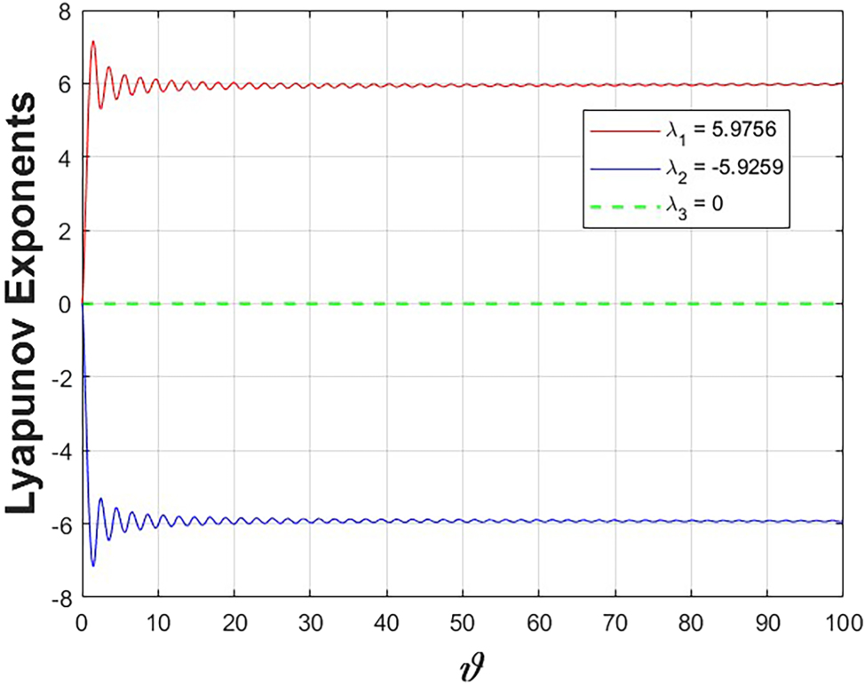
Demonstration of Lyapunov exponent profile for Eq. (19) where q = 2.3, m = 1.5, l = −0.8, A = 1.3, B = 3.6 with the initial state
An overview of the successive Lyapunov exponent procedure.
| Time | λ 1 | λ 2 | λ 3 |
|---|---|---|---|
| 10 | 6.0429 | −6.0377 | 0.0000 |
| 20 | 6.0178 | −6.0074 | 0.0000 |
| 30 | 5.9858 | −5.9704 | 0.0000 |
| 40 | 5.9632 | −5.9428 | 0.0000 |
| 50 | 5.942 | −5.9165 | 0.0000 |
| 60 | 5.9332 | −5.9028 | 0.0000 |
| 70 | 5.9329 | −5.8975 | 0.0000 |
| 80 | 5.9415 | −5.9013 | 0.0000 |
| 90 | 5.9586 | −5.9136 | 0.0000 |
| 100 | 5.9756 | −5.9259 | 0.0000 |
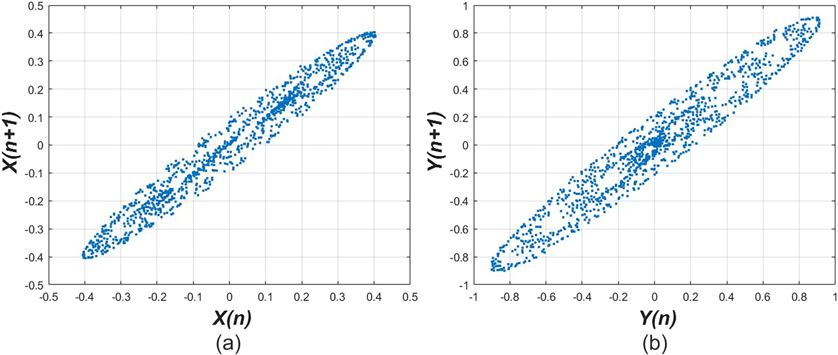
Demonstration of return map profile for Eq. (19) where, q = 2.3, m = 1.5, l = −0.8, A = 1.3, B = 3.6 with initial state
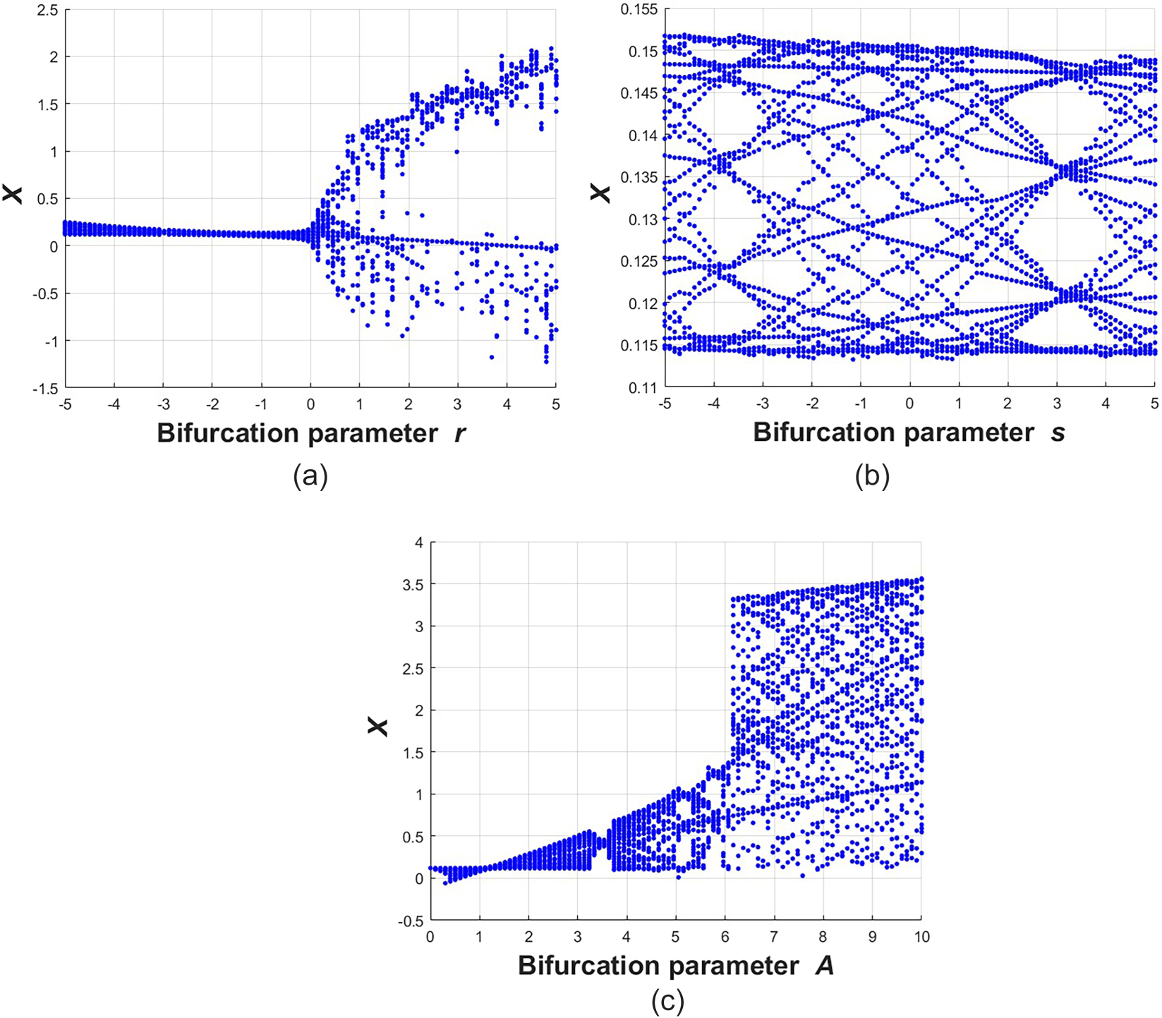
Demonstration of bifurcation profile for Eq. (19) where q = 2.3, m = 1.5, l = −0.8, A = 1.3, B = 3.48 with the initial state
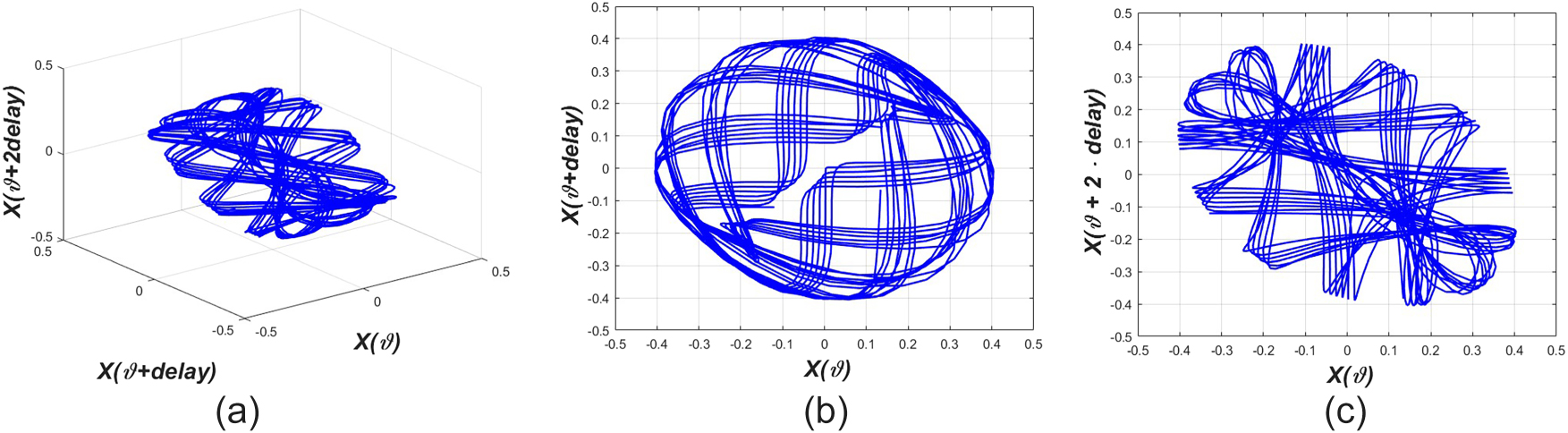
Demonstration of the strange attractor profile for Eq. (19), where q = 2.3, m = 1.5, l = −0.8, A = 1.3, B = 3.6 with the initial state

Demonstration of the strange attractor plot for Eq. (19), where q = 2.3, m = 1.5, l = −0.8, A = 1.3, B = 3.6 with the initial state
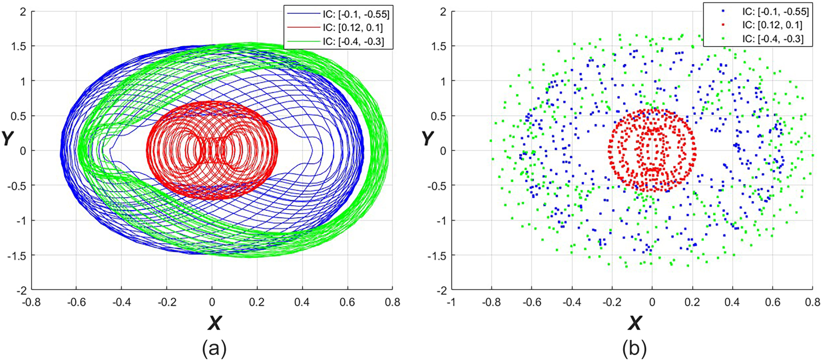
Demonstration of 2D phase plot and Poincaré plot of multistability for Eq. (19), where q = 2.3, m = 1.5, l = −0.8, A = 1.3, B = 3.6 with the initial state
7 Novelty of the results
The uniqueness of this work is discussed in this part. Three recently published papers are considered to prove the novelty of this work [41], [42], [43]. Abubakar and Asif used the ϕ
6-model expansion method to solve the Z model and obtain topological solutions [41]. In addition, Kalim and his co-author utilized the extended hyperbolic function process and the unified procedure in the governing framework, obtaining kink waveforms, periodic shapes, and dark solitons [42]. Moreover, Zhao and Tianyong provided some dynamic designs: breather wave and dark soliton by applying the bifurcation technique and the generalized
The outcomes of this work reveal some unique dynamical patterns, including bright solitons, kink and anti-kink waveforms, singular breathers, and multiple breathers. Additionally, stability analysis for equilibrium points and diverse approaches for identifying chaos were discussed in this study. Thus, this work offers some unique and finer outcomes than the abovementioned papers.
To clearly understand, Table 2 highlights the comparison of our study with Batool et al.’s [44] and Motsepa et al.’s [45] work.
| Aspect | Our investigation | Batool et al.’s [44] work | Motsepa et al.’s [45] work |
|---|---|---|---|
| Studied model | Zoomeron model | Zoomeron model | Zoomeron model |
| Executed procedure | The modified Kudrynshov and the modified alternative
|
The extended
|
The Lie symmetries are applied to obtain group-invariant solutions |
| Categories of solutions | Hyperbolic, trigonometric, logarithmic, exponential, and rational solutions with bright solitons, localized waves, singular breather waves, kink and anti-kink patterns, and multi-breather waveforms. | Hyperbolic, trigonometric, and rational solutions with some kink and singular solutions. | Exponential and Jacobi-type solutions. |
| Stability of equilibrium points | Investigate the stability of equilibrium points | Not studied the equilibrium points | Not studied the equilibrium points |
| Chaos detecting processes | Return maps, Lyapunov exponents, strange attractors, and multistability to confirm the presence of chaotic patterns in the suggested model. | Not analyzed the Chaotic nature | Not analyzed the Chaotic nature |
| Graph type | Three-dimensional, density, and two-dimensional curves with imaginary, real, and absolute values of the solutions | Used only 3D and contour plots. | Not used any types of plots. |
| Area of investigation | Highlights diverse domains, including soliton dynamics, attractors, fractal dimensions, chaos theory, and multistability analysis. | Discussed only soliton phenomena. | Discussed only group-invariant solutions. |
8 Limitations of the employed analytical techniques
This research employs two analytical techniques, which offer important details about the diverse dynamics of solitons in hyperbolic, trigonometric, logarithmic, exponential, and rational solutions within the Zoomeron model. These solutions include bright solitons, localized waves, singular breather waves, kink and anti-kink patterns, and multi-breather waveforms. However, these two methods possess some limitations. Our employed methods need proper variable transformation and the balance rule. It requires a particular initial solution, an auxiliary equation, and parameter values. The methods provide only limited analytical solutions, which must be verified numerically. These two techniques do not describe multi-soliton interactions, stability, bifurcations, chaotic nature, and other dynamical behaviors. Additionally, by applying these two processes, we obtain a system of algebraic equations that requires solving using computational software like Maple, Mathematica, etc., and in some specific cases, this software cannot solve it.
9 Conclusions
In this paper, the modified alternatives
Acknowledgments
Thanks to the editor and anonymous reviewers for their procedural support.
-
Funding information: The authors state no funding is involved.
-
Author contributions: Tarmizi Usman: Methodology, software, wrote the original draft; Noor Alam: Methodology, Software, wrote the original draft; Mohammad Safi Ullah: conceptualization, supervision, validation; Miguel Vivas-Cortez: writing– review and editing, resources, acquisition, Muhammad Abbas: resources, writing– review and editing, formal analysis; Shailendra Singh: writing– review and editing, visualization, investigation, formal analysis. All authors have accepted responsibility for the entire content of this manuscript and approved its submission.
-
Conflict of interest: The authors state no conflict of interest.
-
Data availability statement: All data generated or analyzed during this study are included in this published article.
References
1. Mostafa, M, Ullah, MS. Soliton outcomes and dynamical properties of the fractional Phi-4 equation. AIP Adv 2025;15:015105. https://doi.org/10.1063/5.0245261.Suche in Google Scholar
2. Seadawy, AR, Bilal, M, Younis, M, Rizvi, STR, Althobaiti, S, Makhlouf, MM. Analytical mathematical approaches for the double-chain model of DNA by a novel computational technique. Chaos Solitons Fract 2021;144:110669. https://doi.org/10.1016/j.chaos.2021.110669.Suche in Google Scholar
3. Roshid, MM, Rahman, MM, Roshid, HO, Bashar, MH. A variety of soliton solutions of time M-fractional: Non-linear models via a unified technique. PLoS One 2024;19:e0300321. https://doi.org/10.1371/journal.pone.0300321.Suche in Google Scholar PubMed PubMed Central
4. Baskonus, HM, Guirao, JLG, Kumar, A, Causanilles, FSV, Bermudez, GR. Regarding new traveling wave solutions for the mathematical model arising in telecommunications. Adv Math Phys 2021;2021:5554280–11. https://doi.org/10.1155/2021/5554280.Suche in Google Scholar
5. Bishop, AR. Solitons in condensed matter physics. Phys Scr 1979;20:409–23. https://doi.org/10.1088/0031-8949/20/3-4/016.Suche in Google Scholar
6. Alam, N, Poddar, S, Karim, ME, Hasan, MS, Lorenzini, G. Transient MHD radiative fluid flow over an inclined porous plate with thermal and mass diffusion: an EFDM numerical approach. Math Mod Eng Prob 2021;8:739–49. https://doi.org/10.18280/mmep.080508.Suche in Google Scholar
7. Seadawy, AR, Arshad, M, Lu, D. The weakly nonlinear wave propagation theory for the Kelvin-Helmholtz instability in magnetohydrodynamics flows. Chaos Solitons Fract 2020;139:110141. https://doi.org/10.1016/j.chaos.2020.110141.Suche in Google Scholar
8. Ma, WX, Lee, JH. A transformed rational function method and exact solutions to the 3+1 dimensional Jimbo–Miwa equation. Chaos Solitons Fract 2009;42:1356–63. https://doi.org/10.1016/j.chaos.2009.03.043.Suche in Google Scholar
9. Shukla, VK, Joshi, MC, Mishra, PK, Xu, C. Adaptive fixed-time difference synchronization for different classes of chaotic dynamical systems. Phy Scri 2024;99:095264. https://doi.org/10.1088/1402-4896/ad6ec4.Suche in Google Scholar
10. Mahmud, AA, Tanriverdi, T, Muhamad, KA. Exact traveling wave solutions for (2+1)-dimensional Konopelchenko-Dubrovsky equation by using the hyperbolic trigonometric functions methods. Int J Math Comput Eng 2023;1:11–24. https://doi.org/10.2478/ijmce-2023-0002.Suche in Google Scholar
11. Alam, N, Ma, WX, Ullah, MS, Seadawy, AR, Akter, M. Exploration of soliton structures in the Hirota–Maccari system with stability analysis. Mod Phys Lett B 2025;39:2450481. https://doi.org/10.1142/s0217984924504815.Suche in Google Scholar
12. Zhang, H, Manafian, J, Singh, G, Ilhan, OA, Zekiy, AO. N-lump and interaction solutions of localized waves to the (2 + 1)-dimensional generalized KP equation. Results Phys 2021;25:104168. https://doi.org/10.1016/j.rinp.2021.104168.Suche in Google Scholar
13. Alam, N, Ullah, MS, Nofal, TA, Ahmed, HM, Ahmed, KK, AL-Nahhas, MA. Novel dynamics of the fractional KFG equation through the unified and unified solver schemes with stability and multistability analysis. Nonlin Eng 2024;13:20240034. https://doi.org/10.1515/nleng-2024-0034.Suche in Google Scholar
14. Lin, J, Xu, C, Xu, Y, Zhao, Y, Pang, Y, Liu, Z, et al.. Bifurcation and controller design in a 3D delayed predator-prey model. AIMS Math 2024;9:33891–929. https://doi.org/10.3934/math.20241617.Suche in Google Scholar
15. Ullah, MS, Seadawy, AR, Ali, MZ, Roshid, HO. Optical soliton solutions to the Fokas–Lenells model applying the φ6-model expansion approach. Opt Quant Electron 2023;55:495. https://doi.org/10.1007/s11082-023-04771-3.Suche in Google Scholar
16. Ullah, MS, Baleanu, D, Ali, MZ, Roshid, HO. Novel dynamics of the Zoomeron model via different analytical methods. Chaos Solitons Fract 2023;174:113856. https://doi.org/10.1016/j.chaos.2023.113856.Suche in Google Scholar
17. Ma, WX. A novel kind of reduced integrable matrix mKdV equations and their binary Darboux transformations. Mod Phys Lett B 2022;36:22500944. https://doi.org/10.1142/s0217984922500944.Suche in Google Scholar
18. Kumar, S, Nisar, KS, Kumar, A. A (2+1)-dimensional generalized Hirota–Satsuma–Ito equations: lie symmetry analysis, invariant solutions and dynamics of soliton solutions. Results Phys 2021;28:104621. https://doi.org/10.1016/j.rinp.2021.104621.Suche in Google Scholar
19. Akbar, MA, Ali, NHM, Din, STM. The modified alternative G′/G-expansion method to nonlinear evolution equation: application to the (1+1)-dimensional Drinfel’d-Sokolov-Wilson equation. Spri Plus 2013;2:327.10.1186/2193-1801-2-327Suche in Google Scholar PubMed PubMed Central
20. Hosseini, K, Alizadeh, F, Hinçal, E, Kaymakamzade, B, Dehingia, K, Osman, MS. A generalized nonlinear Schrödinger equation with logarithmic nonlinearity and its Gaussian solitary wave. Opt Quant Electron 2024;56:929.10.1007/s11082-024-06831-8Suche in Google Scholar
21. Lu, J. New exact solutions for Kudryashov–Sinelshchikov equation. Adv Differ Equ 2018;2018:374. https://doi.org/10.1186/s13662-018-1769-6.Suche in Google Scholar
22. Nguyen, AT, Nikan, O, Avazzadeh, Z. Traveling wave solutions of the nonlinear Gilson–Pickering equation in crystal lattice theory. J Ocean Eng Sci 2024;9:40–9. https://doi.org/10.1016/j.joes.2022.06.009.Suche in Google Scholar
23. Demiray, S, Ünsal, O, Bekir, A. New exact solutions for Boussinesq type equations by using G′/G,1/G and 1/G-expansion methods. Acta Phys Polo A 2014;125:1093–8.10.12693/APhysPolA.125.1093Suche in Google Scholar
24. Shukla, VK, Joshi, MC, Mishra, PK, Xu, C. Mechanical analysis and function matrix projective synchronization of El-Nino chaotic system. Phy Scri 2024;100:015255. https://doi.org/10.1088/1402-4896/ad9c28.Suche in Google Scholar
25. San, S, Altunay, R. Application of the generalized Kudryashov method to various physical models. Appl Math Inf Sci Lett 2021;8:7–13.Suche in Google Scholar
26. Alam, N, Akbar, A, Ullah, MS, Mostafa, M. Dynamic waveforms of the new Hamiltonian amplitude model using three different analytic techniques. Indian J Phys 2025;99:2125–32. https://doi.org/10.1007/s12648-024-03426-7.Suche in Google Scholar
27. Khan, A, Saifullah, S, Ahmad, S, Khan, MA, Rahman, M. Dynamical properties and new optical soliton solutions of a generalized nonlinear Schrödinger equation. Eur Phys J Plus 2023;138:1059. https://doi.org/10.1140/epjp/s13360-023-04697-5.Suche in Google Scholar
28. Cui, Q, Xu, C, Xu, Y, Ou, W, Pang, Y, Liu, Z, et al.. Bifurcation and controller design of 5D BAM neural networks with time delay. Int J Numer Model: Electron Net Dev Field 2024;37:e3316. https://doi.org/10.1002/jnm.3316.Suche in Google Scholar
29. Khaliq, S, Ullah, A, Ahmad, S, Akgül, A, Yusuf, A, Sulaiman, TA. Some novel analytical solutions of a new extented (2+1)-dimensional Boussinesq equation using a novel method. J Ocean Eng Sci 2022;10:19.10.1016/j.joes.2022.04.010Suche in Google Scholar
30. Zhoa, Y, Xu, C, Xu, Y, Lin, J, Pang, Y, Liu, Z, et al.. Mathematical exploration on control of bifurcation for a 3D predator-prey model with delay. AIMS Math 2024;9:29883–915. https://doi.org/10.3934/math.20241445.Suche in Google Scholar
31. Ganie, AH, AlBaidani, MM, Wazwaz, AM, Ma, WX, Shamima, U, Ullah, MS. Soliton dynamics and chaotic analysis of the Biswas–Arshed model. Opt Quant Electron 2024;56:1379. https://doi.org/10.1007/s11082-024-07291-w.Suche in Google Scholar
32. Khaliq, S, Ahmad, S, Ullah, A, Ahmad, H, Saifullah, S, Nofal, TA. New waves solutions of the (2+1)-dimensional generalized Hirota–Satsuma–Ito equation using a novel expansion method. Results Phys 2023;50:106450. https://doi.org/10.1016/j.rinp.2023.106450.Suche in Google Scholar
33. Ganie, AH, Rahaman, MS, Aladsani, FA, Ullah, MS. Bifurcation, chaos, and soliton analysis of the Manakov equation. Nonlin Dyn 2025;113:9807–21. https://doi.org/10.1007/s11071-024-10829-y.Suche in Google Scholar
34. Khalifa, AS, Badra, NM, Ahmed, HM, Rabie, WB. Retrieval of optical solitons in fiber Bragg gratings for high-order coupled system with arbitrary refractive index. Optik 2023;287:171116. https://doi.org/10.1016/j.ijleo.2023.171116.Suche in Google Scholar
35. Roshid, MM, Rahman, MM. Bifurcation analysis, modulation instability and optical soliton solutions and their wave propagation insights to the variable coefficient nonlinear Schrödinger equation with Kerr law nonlinearity. Nonlin Dyn 2024;112:16355–77. https://doi.org/10.1007/s11071-024-09872-6.Suche in Google Scholar
36. Roshid, MM, Abdalla, M, Osman, MS. Dynamical analysis of Jacobian elliptic function soliton solutions, and chaotic behavior with defective tools of the stochastic PNLSE equation with multiplicative white noise. Chaos Solitons Fract 2025;201:117288. https://doi.org/10.1016/j.chaos.2025.117288.Suche in Google Scholar
37. Almheidat, M, Alqudah, M, Alderremy, AA, Elamin, M, Mahmoud, EE, Ahmad, S. Lie-bäcklund symmetry, soliton solutions, chaotic structure and its characteristics of the extended (3 + 1) dimensional Kairat-II model. Nonlin Dyn 2025;113:2635–51. https://doi.org/10.1007/s11071-024-10325-3.Suche in Google Scholar
38. Islam, SMR, Khan, K, Akbar, MA. Optical soliton solutions, bifurcation, and stability analysis of the Chen-Lee-Liu model. Results Phys 2023;51:106620. https://doi.org/10.1016/j.rinp.2023.106620.Suche in Google Scholar
39. Riaz, MB, Jhangeer, A, Duraihem, FZ, Martinovic, J. Analyzing dynamics: lie symmetry approach to bifurcation, chaos, multistability, and solitons in extended (3 + 1)-dimensional wave equation. Symmetry 2024;16:608. https://doi.org/10.3390/sym16050608.Suche in Google Scholar
40. Alam, N, Ullah, MS, Manafian, J, Mahmoud, KH, Alsubaie, AS, Ahmed, HM, et al.. Bifurcation analysis, chaotic behaviors, and explicit solutions for a fractional two-mode Nizhnik-Novikov-Veselov equation in mathematical physics. AIMS Math 2025;10:4558–78. https://doi.org/10.3934/math.2025211.Suche in Google Scholar
41. Isah, MA, Yokus, A. Nonlinear dispersion dynamics of optical solitons of Zoomeron equation with new φ6-model expansion approach. J Vibrat Test Syst Dyn 2024;8:2–25.10.5890/JVTSD.2024.09.002Suche in Google Scholar
42. Tariq, KU, Liu, JG, Nisar, S. Study of explicit travelling wave solutions of nonlinear (2 + 1)-dimensional Zoomeron model in mathematical physics. J Nonlin Comp Data Sci 2024;25:109–24. https://doi.org/10.1515/jncds-2023-0068.Suche in Google Scholar
43. Li, Z, Han, T. Bifurcation and exact solutions for the (2 + 1)-dimensional conformable time-fractional Zoomeron equation. Adv Differ Equ 2020;2020:1–13.10.1186/s13662-020-03119-5Suche in Google Scholar
44. Batool, F, Akram, G, Sadaf, M, Mehmood, U. Dynamics investigation and solitons Formation for (2 + 1) -dimensional zoomeron equation and foam drainage equation. J Nonlin Math Phy 2023;30:628–45.10.1007/s44198-022-00097-ySuche in Google Scholar
45. Motsepa, T, Khalique, CM, Gandarias, ML. Symmetry analysis and conservation laws of the Zoomeron equation. Symmetry 2017;9:27. https://doi.org/10.3390/sym9020027.Suche in Google Scholar
© 2026 the author(s), published by De Gruyter, Berlin/Boston
This work is licensed under the Creative Commons Attribution 4.0 International License.
Artikel in diesem Heft
- Research Articles
- The dynamics of prey–predator model with global warming on carrying capacity and wind flow on predation
- Analysis of traffic density dynamics under varied noise conditions using data-driven partial differential equations
- Soliton, stability, multistability, and diverse tools for identifying chaos in a nonlinear model with two modified methods
- An efficient recurrent neural network based confusion component construction and its application in protection of saliency in digital information
- SI Nonlinear Analysis and Design of Communication Networks for IoT Appl.APC
- A passive wireless sensor signal anti-interference method based on RFID
- SI: Advances in Nonlinear Dynamics and Control APC
- Application of backpropagation neural network algorithm in e-commerce customer churn prediction