Numerical simulation of Burgers’ equation using cubic B-splines
-
C. Lakshmi


Abstract
In this paper, a numerical θ scheme is proposed for solving nonlinear Burgers’ equation. By employing Hopf-Cole transformation, the nonlinear Burgers’ equation is linearized to the linear Heat equation. The resulting Heat equation is further solved by cubic B-splines. The time discretization of linear Heat equation is carried out using Crank-Nicolson scheme
1 Introduction
Consider the nonlinear Burgers’ equation given by
where
with initial condition
and boundary conditions
where ν > 0 is the kinematic viscosity parameter and g, f1 and f2 are given functions of the arguments which are sufficiently smooth.
Burgers’ equation is one of the most fundamental nonlinear partial differential equations which has its impact in numerous areas of scientific research such as viscous flow and turbulence, gas dynamics, shock theory, traffic flow, stochastic process, cosmology, etc. Burgers’ equation was introduced in 1915 by a British-American mathematician Harry Bateman [6]. He was interested in vanishing the viscosity limit, i.e. ν →0. The applications of Burgers’ equation began when a Dutch physicist J. M. Burger [7] made use of it to elucidate some important characteristics of turbulence such as balance of energy and appearance of dissipation layers. He did immense research in this equation and to honour his contributions, this equation is well known as Burgers’ equation. Research in Burgers’ equation became more rigorous when Hopf [8] and Cole [9] in 1950 and 1951 respectively, independently developed a nonlinear transformation which could map the nonlinear Burgers’ equation to a linear Heat equation. Thus the analytical solution of Burgers’ equation could be obtained for a restricted set of initial conditions. Burgers’ equation, due to the simultaneous presence of convective term
Burgers’ equation is basically the Navier Stokes equation without the pressure term. For low kinematic viscosity there can be velocity discontinuities, i.e. shocks. Kreiss and Kreiss [10] considered the viscous Burgers’ equation with the initial and non-homogeneous Dirichlet boundary conditions to study the effect of shock on convergence of steady state solution. They proved that to speed up the convergence to the steady state, the shock should be located at the boundary. On the other hand, location of shock in the interior leads to very slow convergence. The speed of convergence was studied by analyzing the corresponding eigenvalue problem. Bec and Khanin [11] explained Burgers’ turbulence as the study of solutions to the one or multi-dimensional Burgers’ equation with random initial conditions or random forcing. Recently, it has become a point of attraction to many researchers due to the new emerging application of Burgers’ model to statistical physics, cosmology and fluid dynamics.
One of the earliest attempts to solve Burgers’ equation was by Benton and Platzman [12] who presented 35 distinct analytic solutions of the equation with different initial conditions. Rodin [13] studied some approximate and exact solution of boundary value problems for Burgers’ equation with the help of Hopf-Cole transformation. Varoglu and Finn [14] developed a finite element method based on weighted residual method where the method of characteristic was employed using space time elements. Cadwell et al. [15] attempted a piecewise approximation method (finite element method) using two elements with the aim of ‘chasing the peak’ by altering the size of the elements at each stage by using the information at the previous step. Cadwell and Smith [16] extended this method to the general case of n elements. They observed that for large Reynold’s number, the finite element results were much superior to the finite difference results. A number of other authors used moving node finite element method to solve Burgers’ equation. Gelinas et al. [17] presented a node moving finite element method which can be applied to large gradients or shocks with high resolution and accuracy. In their system, the nodes move systematically and continuously to those regions where they are required the most. Cadwell et al. [18] further developed a moving node finite element method by using an algorithm which was a generalization of that considered by Caldwell et al. [15]. Several other finite element techniques were employed for solving Burgers’ equation [19], [20], [2]. Asaithambi [21] presented a simple numerical method based on automatic differentiation or algorithmic differentiation that used second-order finite-differences for the spatial derivatives and marched the solution in time using a Taylor series expansion. Kadalbajoo et al. [22] developed an implicit scheme for solving Burgers’ equation. They used a standard backward Euler scheme with constant time step to discretize in temporal direction and a standard upwind finite difference scheme to discretize in spatial direction on piecewise uniform mesh. The quasi-linearization process was used to tackle the nonlinearity. A numerical method based on Crank-Nicolson scheme was put forward by Kadalbajoo and Awasthi [23], where they first reduced the Burgers’ equation to a linear Heat equation using Hopf-Cole transformation and then dicsretized using Crank-Nicolson scheme. The mesh size could be chosen without any restriction. It was shown that the scheme was second order accurate in both space and time and also unconditionally stable. Rashidi et al. [24] proposed the homotopy perturbation method (HPM) for solving generalized Burgers’ and Burger-Fisher equations. In most cases, the method gave good results even with a few terms. Rashidi et al. [25] also employed the homotopy analysis method (HAM) effectively to Burgers’ equation and regularized long wave (RLW) equations and made a comparative study of their results with the HPM to establish the effectiveness of the former method over the latter. Rashidi and Erfani [26] then extended the differential transform method (DTM) to develop approximate analytical solutions of the Burgers’ equation and found that the results were more accurate as compared to HAM. Adomian’s decomposition method was tried by Abbasbandy and Darvishi [27], [28]. Several mesh free methods [29], [30], [31], [32] have also been developed for solving Burgers’ equation. In 2015, Vijitha Mukundan and Ashish Awasthi [33] presented new efficient numerical techniques for solving Burgers’ equation. They used Hopf-Cole transformation to get one-dimensional diffusion equation which was semi-discretized by using method of lines (MOL). Resulting system of ODEs was solved by backward differentiation formulas (BDF) of order one, two and three.
Inan and Bahadir [34] solved the nonlinear Burgers’ equation using an explicit exponential finite difference method. They employed Hopf-Cole transformation to convert the nonlinear Burgers’ equation to linear Heat equation. Inan and Bahadir [35] further illustrated an implicit and a fully implicit exponential finite difference method for solving Burgers’ equation. They used Newton’s method to solve the nonlinear system at each time step. Inan and Bahadir [36] improved on their exponential method which lead to Crank-Nicolson exponential finite difference solution of Burgers’ equation. In this method, they used Crank-Nicolson scheme for discretization and Newton Raphson method to solve the system at each time step. Recently in 2015, Inan and Bahadir [37] came up with an alternate implicit and Crank-Nicolson exponential finite difference method where they first reduced the Burgers’ equation to linear Heat equation by Hopf-Cole transformation and then solved the same using implicit and Crank-Nicolson exponential finite difference method.
A remarkable method to solve Burgers’ equation is by using splines. The term ‘splines’ is adopted from the name of a flexible strip of metal used by drafters in olden times to assist in drawing curves. Usage of spline functions has great advantages. They are constructed in such a way that they possess high degree of smoothness even at the juncture between two polynomial pieces, i.e. nth degree spline function is continuous up to (n - 1)th derivative. They are easy to store, manipulate and evaluate on a digital computer. The matrices arising naturally on using splines have convenient determinantal properties. Moreover, every continuous function on the interval [a, b]can be approximated arbitrarily well by polynomial splines, provided a sufficient number of knots are allowed. These desirable properties of splines have driven researchers to develop different types of spline functions of various degree. B-spline or Basis spline is a spline function that has minimal support with respect to given degree of smoothness and domain partition. Any spline function of a particular degree and smoothness can be written as a linear combination of B-splines of the same degree and smoothness. A remarkable property of B-spline that it has minimal support bestows it with a computational edge over finite element method, while its fourth order accuracy marks it superior to finite difference methods.
Splines was used in a mathematical context for the first time in 1946 by I. J. Schoenberg [38], in connection with smooth piecewise polynomial approximation. Since then, it has come a long way in solving Burgers’ equation. B-spline was also introduced by Schoenberg to approximate equidistant data by analytic functions by means of integrals. B-splines for arbitrarily spaced data was later given by Curry and Schoenberg [39]. Roach and Yanping [40] used linear exponential spline function as an interpolant to generate finite difference representation of Burgers’ equation. The time marching was performed using backward Euler method. In 1992, L.R.T. Gardner et al. [41] developed a collocation solution of Burgers’ equation using cubic B-spline finite element method. Kutluay et al. [42] presented a least-squares quadratic B-spline finite element method for Burgers’ equation by applying the classical weighted residual method over the finite elements. Dag et. al [43] solved time split and space split Burgers’ equation using B-spline collocation method. Aksan [44] brought forward another method in which Burgers’ equation was converted to a set of nonlinear ordinary differential equations by the method of discretization in time and then each of them was solved by applying the quadratic B-spline finite element method. A numerical solution based on collocation using septic splines was developed by Ramadan et al. [45]. Here, the time discretization was done using Crank-Nicolson scheme. The method proved to be unconditionally stable. Ramadan et al. [46] also proposed a non-polynomial spline solution of Burgers’ equation. The non-polynomial spline function in this work has a trigonometric part and a polynomial part of first degree. The C∞ differentiability of the trigonometric part of non-polynomial spline compensates for the loss of smoothness inherited by polynomial splines. Moving boundary conditions were used to improve the accuracy. In another study of Burgers’ equation by Saka et al. [47], time and space splitting techniques were applied to the Burgers’ equation and the modified Burgers’ equation and then collocation procedure using quintic B-spline was employed to approximate the resulting systems. The method was proven to be better than quadratic B-spline F.E.M and quartic B-spline collocation method. Many other numerical methods for solving Burgers’ equation using splines were developed such as that by Jiang and Wang[48], etc. In 2012, R.C. Mittal and R.K. Jain [49] developed a method for solving Burgers’ equation based on collocation of modified cubic B-splines over finite elements. In 2014, Geetha Arora and Brajesh Kumar [50] used modified cubic B-splines in differential quadrature method to give a system of ordinary differential equation, which was solved by strong stability preserving time stepping Runge Kutta (SSP-RK43) scheme.
In this paper, we reduce the Burgers’ equation to a linear Heat equation using Hopf-Cole transformation. Linear Heat equation thus obtained is further solved using cubic B-splines in space. Time discretization is done using both Crank-Nicolson scheme as well as backward Euler scheme. We have considered various test examples and computed L2 and L∞ error norms to establish the accuracy of the proposed methods. Stability check using Von Neumann stability analysis has confirmed that the method is unconditionally stable. We have also compared our numerical results with those of Kutluay et al. [1], Ozis et al. [2], Dag et al. [3], Salkuyeh et al. [4] and Korkmaz et al. [5] and established that our results are more accurate as compared to the above mentioned works.
2 Hopf-Cole Transformation
Hopf [8] and Cole [9] in 1950 and 1951 respectively came up with a nonlinear transformation which could reduce the Burgers’ equation to a linear Heat equation for a restricted set of initial conditions. The transformation was thus named after them as Hopf-Cole transformation. The concept of Hopf-Cole transformation is of prime significance in the theory of conservation laws. Hopf and Cole proved that in the context with initial and boundary conditions of Eq. (1.1a), the nonlinear transformation
satisfies the viscous Burgers’ equation
where ϕ(x, t) is a solution to the linear Heat equation
Therefore, by using the nonlinear Hopf-Cole transformation, the nonlinear Burgers’ equation Eq. (1.1a) with initial condition Eq. (1.1b) and Dirichlet boundary conditions (f1(t) = f2(t) = 0, 0 ≤ t ≤ Τ ) is reduced to linear Heat equation
with initial condition
and boundary conditions
3 Exact solution of Burgers’ equation
The Fourier series solution to the linearized Heat equation is
with Fourier coefficients at t = 0 as
Using the Hopf-Cole transformation the exact solution to Burgers’ equation Eq. (1.1a) is
4 Numerical θ scheme based on cubic B-splines
Consider a uniform partition of the solution domain [a, b] with nodal points xj as a = x0 < x1 < ... < xN = b. The cubic B-spline at the nodal points is given by
where, B-1, B0, ..., BN-1, BN, BN+1 forms a basis of all cubic continuous functions over [a, b]. Thus, any cubic continuous function on [a, b] can be written as a linear combination of the cubic B-splines as
where δm(t), m = -1,..., N + 1 are the time dependent parameters to be obtained from boundary conditions and B-spline formulation. It may be noted that each cubic B-spline is non-zero over four adjacent intervals.
The values of Bj(x)and its derivatives obtained from Eq. (4.1) are tabulated in Table 1.
Coefficient of cubic B-spline and its derivatives at nodal points xj
| χ | χj-2 | χj-1 | χj | χj+1 | χj+2 |
|---|---|---|---|---|---|
| Bj(χ) | 0 | 1 | 4 | 1 | 0 |
| 0 | 0 | 0 | |||
| 0 | 0 |
Using approximation function Eq. (4.2) and Table 1, we have
The linear Heat equation Eq. (2.2) with initial condition Eq. (2.3) and boundary condition Eq. (2.4) is to be solved by making use of cubic B-spline.
To begin with, consider the weighted average of linear Heat equation as follows:
In this paper, we make use of Crank-Nicolson scheme, i.e.
Discretizing time derivative of Eq. (4.6) by finite difference
Substituting Eq. (4.3) and Eq. (4.5) in Eq. (4.7), we have
The parameters δ-1 and δΝ+1in Eq. (4.8) are eliminated using boundary condition as follows:
From Eq. (4.4) and boundary conditions Eq. (2.4), we have
The initial vector δ0, i.e.
The accuracy in temporal direction is improved by Richardson extrapolation as follows:
where h and k are the grid lengths in x and t directions respectively.
5 Stability Analysis
The stability analysis is investigated using a versatile technique known as Fourier stability method. Using this method, we assume
where ζ is known as amplification factor. For stability we require ζ < 1.
Using Eq. (5.1) it follows that
Substituting Eq. (5.1) to Eq. (5.4) in Eq. (4.8), we get
Dividing through out by ζneiαm
Putting eiα = cos α+ i sin αand e-iα = cos α - i sin α
Simplifying Eq. (5.7) we get;
By Fourier stability method, solution is stable for ζ < 1.
For simplifying the notation, we put
To prove that
When θ = 1;
so that Eq. (5.9) reduces to
Here,
Hence a ≤ b and therefore
When
In this case,
Hence a ≤ b and therefore ζ ≤ 1.
Hence, for both values of Θ, the scheme is unconditionally stable.
6 Numerical Experiments and Discussion
In this section, we consider some test examples to demonstrate the efficiency and accuracy of the proposed method. The numerical solutions obtained by proposed method at various times and for different values of coefficients of viscosity are plotted in the cases when θ = 0.5 and θ = 1 and compared with exact solution. The accuracy and efficiency of the method for each example considered is examined by calculating the L2 and L∞ error norms which are defined as follows:
where
The 2-D plots and surface plots have been plotted to confirm the numerical results. The numerical results have also been compared with those of Kutluay et al. [1], Ozis et al. [2], Dag et al. [3], Salkuyeh et al. [4] and Korkmaz et al. [5] When
and when θ = 1, the system of equation Eq. (4.8) reduces to
Consider the Burgers’ equation Eq. (1.1a) with the initial condition
and the homogeneous boundary conditions
By Hopf-Cole transformation Eq. (2.1), the Burgers’ equation is transformed to the linear Heat equation Eq. (2.2) with the initial condition:
and Neumann type boundary conditions,
Using the method of separation of variable the (exact) Fourier series solution to the above linearized problem defined by Eq. (2.2) with initial and boundary conditions given by Eq. (6.6) and Eq. (6.7) respectively can be obtained as
with the Fourier coefficients
The exact solution of the problem is given by Eq. (3.1) with A0 and An defined as in Eq. (6.9) and Eq. (6.10), respectively.
In order to solve the systems (6.2) and (6.3) numerically, a starting value of δ0, i.e.
Also,
We finally arrive at the solution of Burgers’ equation by substituting solution of linear Heat equation in Eq. (4.11).
Considering Burgers’ equation Eq. (1.1a) with initial condition
and boundary condition
By Hopf-Cole transformation Eq. (2.1) the Burgers’ equation is transformed to the linear Heat equation Eq. (2.2) with the initial condition
and Neumann type boundary conditions
The exact solution of this problem is obtained in a similar way as in Example 1. It may be noted that the Fourier coefficients A0 and An are the following:
Numerical solution may also be obtained in a similar way as in Example 1. In this case, the starting value of δ0, i.e.
Consider the Burgers’ equation Eq. (1.1a) with the initial condition
and homogeneous boundary conditions
where, σ > 0 is a parameter.
By Hopf-Cole transformation, the Burgers’ equation Eq. (1.1a) is transformed to the linear Heat equation Eq. (2.2) with the initial condition
and Neumann type boundary conditions
The exact solution of the above equation is given by
To obtain the numerical solution, the required starting value of δ0, i.e.
In the tables that follow, we have given the L2and L∞ error norms of the examples discussed for different values of coefficient of viscosity (v), time step (Δt) and space step (h) for θ = 0.5 and θ = 1 . We have also presented the comparison of our numerical results with those of Kutluay et al. [1], Ozis et al. [2], Dag et al. [3], Salkuyeh et al. [4] and Korkmaz et al. [5].
Tables 2 to 4 give the L2 and L∞ error norms of Example l for v = 1, 0.1 and 0.01 respectively. The L2 and L∞ error norms of Example 2 are given in Tables 5 to 7 and those of Example 3 are shown in tables 8 to 10. The L2 and L∞ error norms are very small establishing that numerical solution and analytical solution are very close. We have also presented the graphs for numerical solution in comparison with the exact solution for all the examples.
L2 and L∞error norms of Example 1 for ν = 1, ∆t = 0.001 and h = 0.0125
| t | θ = 0.5 | θ=1 | ||
|---|---|---|---|---|
| L2 | L∞ | L2 | L∞ | |
| 0.1 | 3.26483×10⁻⁴ | 2.06493×10⁻³ | 3.30030×10⁻⁴ | 2.08277×10⁻³ |
| 0.2 | 1.39087×10⁻⁴ | 8.79499×10⁻⁴ | 7.25395×10⁻⁵ | 4.58657×10⁻⁴ |
| 0.3 | 5.83493×10⁻⁵ | 3.69059×10⁻⁴ | 8.44307×10⁻⁶ | 5.33990×10⁻⁵ |
| 0.4 | 2.41857×10⁻⁵ | 1.52965×10⁻⁴ | 3.77824×10⁻⁶ | 2.38963×10⁻⁵ |
| 0.5 | 9.92293×10⁻⁶ | 6.27582×10⁻⁵ | 3.99013×10⁻⁶ | 2.52359×10⁻⁵ |
L2 and L∞error norms of Example 1 for ν = 0.1, ∆t = 0.0001 and h = 0.01
| t | θ = 0.5 | θ=1 | ||
|---|---|---|---|---|
| L2 | L∞ | L2 | L∞ | |
| 1 | 2.05415×10⁻⁴ | 1.94686×10⁻³ | 2.95631×10⁻⁴ | 2.39409×10⁻³ |
| 2 | 6.52273×10⁻⁵ | 6.41337×10⁻⁴ | 1.22403×10⁻⁵ | 1.11272×10⁻⁴ |
| 3 | 2.41200×10⁻⁵ | 2.40547×10⁻⁴ | 1.50685×10⁻⁵ | 1.50261×10⁻⁴ |
| 4 | 9.23729×10⁻⁶ | 9.23372×10⁻⁵ | 1.25801×10⁻⁵ | 1.25745×10⁻⁴ |
| 5 | 3.55340×10⁻⁶ | 3.5532×10⁻⁵ | 7.29220×10⁻⁶ | 7.29177×10⁻⁵ |
L2 and L∞ error norms of Example 1 for ν = 0.01, ∆t = 0.005 and h = 0.0125
| t | θ = 0.5 | θ = 1 | ||
|---|---|---|---|---|
| L2 | L∞ | L2 | L∞ | |
| 5 | 1.17747×10⁻⁴ | 5.98388×10⁻⁴ | 4.00832×10⁻⁴ | 1.72249×10⁻³ |
| 10 | 2.79743×10⁻⁵ | 2.05344×10⁻⁴ | 5.50154×10⁻⁵ | 2.98833×10⁻⁴ |
| 15 | 1.74834×10⁻⁵ | 1.20216×10⁻⁴ | 1.60754×10⁻⁵ | 1.00908×10⁻⁴ |
| 20 | 1.05552×10⁻⁵ | 7.29685×10⁻⁵ | 6.28961×10⁻⁶ | 4.26933×10⁻⁵ |
| 25 | 6.57222×10⁻⁶ | 4.59493×10⁻⁵ | 2.68364×10⁻⁶ | 1.87708×10⁻⁵ |
L2 and L∞ error norms of Example 2 for ν = 1, ∆t = 0.0001, h = 0.01
| t | θ = 0.5 | θ = 1 | ||
|---|---|---|---|---|
| L2 | L∞ | L2 | L∞ | |
| 0.1 | 2.83954×10⁻⁴ | 2.00787×10⁻³ | 2.88138×10⁻⁴ | 2.02929×10⁻³ |
| 0.2 | 1.17263×10⁻⁴ | 8.28997×10⁻⁴ | 4.85868×10⁻⁵ | 3.43450×10⁻⁴ |
| 0.3 | 4.79970×10⁻⁵ | 3.39416×10⁻⁴ | 3.50799×10⁻⁶ | 2.47984×10⁻⁵ |
| 0.4 | 1.95002×10⁻⁵ | 1.37889×10⁻⁴ | 9.36010×10⁻⁶ | 6.61869×10⁻⁵ |
| 0.5 | 7.86838×10⁻⁶ | 5.56379×10⁻⁵ | 6.49135×10⁻⁶ | 4.59008×10⁻⁵ |
L2 and L∞ error norms of Example 2 for ν = 0.1, ∆t = 0.001, h = 0.01
| t | θ = 0.5 | θ = 1 | ||
|---|---|---|---|---|
| L2 | L∞ | L2 | L∞ | |
| 1 | 2.60643×10⁻⁴ | 1.80635×10⁻³ | 3.51037×10⁻⁴ | 2.10778×10⁻³ |
| 2 | 9.44114×10⁻⁵ | 6.58582×10⁻⁴ | 3.97978×10⁻⁵ | 2.74071×10⁻⁴ |
| 3 | 3.72652×10⁻⁵ | 2.62888×10⁻⁴ | 2.78606×10⁻⁶ | 1.94185×10⁻⁵ |
| 4 | 1.50501×10⁻⁵ | 1.06392×10⁻⁴ | 7.22900×10⁻⁶ | 5.10839×10⁻⁵ |
| 5 | 6.06745×10⁻⁶ | 4.29058×10⁻⁵ | 5.00608×10⁻⁶ | 3.53980×10⁻⁵ |
L2 and L∞ error norms of Example 2 for ν = 0.01, ∆t = 0.005 and h = 0.005
| t | θ = 0.5 | θ = 1 | ||
|---|---|---|---|---|
| L2 | L∞ | L2 | L∞ | |
| 5 | 5.05467×10⁻⁵ | 5.46951×10⁻⁴ | 5.76664×10⁻⁴ | 3.39188×10⁻³ |
| 10 | 2.35883×10⁻⁵ | 2.16993×10⁻⁴ | 5.54081×10⁻⁵ | 3.87510×10⁻⁴ |
| 15 | 1.14067×10⁻⁵ | 1.06927×10⁻⁴ | 1.05448×10⁻⁵ | 8.37374×10⁻⁵ |
| 20 | 6.22943×10⁻⁶ | 6.01938×10⁻⁵ | 2.03732×10⁻⁶ | 1.76742×10⁻⁵ |
| 25 | 3.66978×10⁻⁶ | 3.61447×10⁻⁵ | 2.49273×10⁻⁷ | 2.50222×10⁻⁶ |
L2 and L∞ error norms of Example 3 for ν = l, ∆t = 0.0001 and h = 0.0125
| t | θ = 0.5 | θ = 1 | ||
|---|---|---|---|---|
| L2 | L∞ | L2 | L∞ | |
| 0.1 | 1.08102×10⁻³ | 6.72107×10⁻³ | 1.08885×10⁻³ | 6.76936×10⁻³ |
| 0.2 | 4.41286×10⁻⁴ | 2.78398×10⁻³ | 2.29689×10⁻⁴ | 1.45036×10⁻³ |
| 0.3 | 1.84079×10⁻⁴ | 1.16382×10⁻³ | 2.66087×10⁻⁵ | 1.68287×10⁻⁴ |
| 0.4 | 7.62220×10⁻⁵ | 4.82117×10⁻⁴ | 1.19130×10⁻⁵ | 7.53275×10⁻⁵ |
| 0.5 | 3.12724×10⁻⁵ | 1.97787×10⁻⁴ | 1.25750×10⁻⁵ | 7.95332×10⁻⁵ |
L2 and L∞ error norms of Example 3 for ν = 0.1, ∆t = 0.001 and h = 0.01
| t | θ = 0.5 | θ = 1 | ||
|---|---|---|---|---|
| L2 | L∞ | L2 | L∞ | |
| 1 | 9.14537×10⁻⁵ | 6.34567×10⁻⁴ | 9.22393×10⁻⁵ | 6.39987×10⁻⁴ |
| 2 | 3.60692×10⁻⁵ | 2.54355×10⁻⁴ | 1.49080×10⁻⁵ | 1.05242×10⁻⁴ |
| 3 | 1.46735×10⁻⁵ | 1.03730×10⁻⁴ | 1.07794×10⁻⁶ | 7.59460×10⁻⁶ |
| 4 | 5.95605×10⁻⁶ | 4.21173×10⁻⁵ | 2.85934×10⁻⁶ | 2.02172×10⁻⁵ |
| 5 | 2.40313×10⁻⁶ | 1.69930×10⁻⁵ | 1.98256×10⁻⁶ | 1.40191×10⁻⁵ |
L2 and L∞ error norms of Example 3 for ν = 0.01, ∆t = 0.005 and h = 0.0125
| t | θ = 0.5 | θ = 1 | ||
|---|---|---|---|---|
| L2 | L∞ | L2 | L∞ | |
| 5 | 1.22382×10⁻⁵ | 7.46116×10⁻⁵ | 1.51129×10⁻⁵ | 9.16912×10⁻⁵ |
| 10 | 7.71923×10⁻⁶ | 4.81380×10⁻⁵ | 7.75865×10⁻⁶ | 4.83819×10⁻⁵ |
| 15 | 5.04586×10⁻⁶ | 3.17368×10⁻⁵ | 4.17679×10⁻⁶ | 2.62915×10⁻⁵ |
| 20 | 3.32657×10⁻⁶ | 2.09931×10⁻⁵ | 2.26833×10⁻⁶ | 1.43235×10⁻⁵ |
| 25 | 2.19179×10⁻⁶ | 1.38506×10⁻⁵ | 1.22415×10⁻⁶ | 7.73911×10⁻⁶ |
In Tables 11 to 13, we have given the comparison of Example 1 at θ = 0.5 and θ = 1 with those of Kutluay et al. [1], Ozis et al [2], Dag et al [3], Salkuyeh et al [4] and Korkmaz et al [5] for Example 1. Tables 14 to 16 give the comparison of numerical results of Example 2 by our method for θ = 0.5 and θ = 1 with those of Kutluay et al [1], Ozis et al [2] and Salkuyeh et al [4]. It can be seen that results by the proposed method are more accurate as compared to the results presented in the above mentioned papers.
Comparison of the numerical solutions of Example 1 for θ = 0.5 and θ = 1 when ν = 1 in comparison with the numerical solutions obtained by Kutluay et al. [1], Korkmaz [5] and Dag [3] for h = 0.0125 and ∆t = 0.0001 and exact solutions
| x | t | [1] | [5] | [3] | θ = 1 | θ = 0.5 | Exact solution |
|---|---|---|---|---|---|---|---|
| 0.25 | 0.4 | 0.01359 | 0.01363 | 0.01355 | 0.013556 | 0.013566 | 0.01357 |
| 0.6 | 0.00189 | 0.00190 | 0.00188 | 0.001886 | 0.001881 | 0.00189 | |
| 0.8 | 0.00026 | 0.00026 | 0.00026 | 0.000262 | 0.000262 | 0.00026 | |
| 1.0 | 0.00004 | 0.00003 | 0.00004 | 0.000036 | 0.000036 | 0.00004 | |
| 0.5 | 0.4 | 0.01927 | 0.01932 | 0.01920 | 0.019226 | 0.019227 | 0.01924 |
| 0.6 | 0.00268 | 0.00269 | 0.00266 | 0.002671 | 0.002671 | 0.00267 | |
| 0.8 | 0.00037 | 0.00037 | 0.00037 | 0.000372 | 0.000371 | 0.00037 | |
| 1.0 | 0.00005 | 0.00005 | 0.00005 | 0.000051 | 0.000051 | 0.00005 | |
| 0.75 | 0.4 | 0.01365 | 0.01363 | 0.01361 | 0.0136250 | 0.0136250 | 0.01363 |
| 0.6 | 0.00189 | 0.00190 | 0.00188 | 0.0018993 | 0.0018892 | 0.00189 | |
| 0.8 | 0.00026 | 0.00026 | 0.00026 | 0.0002624 | 0.0002623 | 0.00026 | |
| 1.0 | 0.00004 | 0.00004 | 0.00004 | 0.0000364 | 0.0000365 | 0.00004 |
Comparison of the numerical solutions of Example 1 for θ = 0.5 and θ = 1 when ν = 1, h = 0.0125, and ∆t = 0.0001 in comparison with the numerical solutions obtained by Ozis et al. [2] and exact solutions
| x | t | [2] | θ = 1 | θ = 0.5 | Exact solution |
|---|---|---|---|---|---|
| 0.25 | 0.1 | 0.25434 | 0.25350 | 0.25350 | 0.25364 |
| 0.15 | 0.15641 | 0.15651 | 0.15652 | 0.15660 | |
| 0.2 | 0.09621 | 0.09638 | 0.09639 | 0.09644 | |
| 0.25 | 0.05904 | 0.05917 | 0.05919 | 0.05921 | |
| 0.5 | 0.1 | 0.37087 | 0.371372 | 0.371373 | 0.37158 |
| 0.15 | 0.22632 | 0.226693 | 0.226703 | .226820 | |
| 0.2 | 0.13812 | 0.138386 | 0.138402 | 0.13847 | |
| 0.25 | 0.08430 | 0.084489 | 0.084496 | 0.08453 | |
| 0.75 | 0.1 | 0.27073 | 0.272436 | 0.272437 | 0.27258 |
| 0.15 | 0.16382 | 0.164279 | 0.164281 | 0.16437 | |
| 0.2 | 0.09915 | 0.099378 | 0.099384 | 0.09943 | |
| 0.25 | 0.06016 | 0.060307 | 0.060317 | 0.06034 |
Comparison of the numerical solutions of Example 1 for θ = 0.5 and θ = lwhenν = 0.1 in comparison with the numerical solutions obtained by Kutluay [1], Ozis [2], Korkmaz [5] and Salkuyeh [4] and exact solutions
| x | t | [1] | [2] | [5] | [4] | θ = 1 | θ = 0.5 | Exact solution |
|---|---|---|---|---|---|---|---|---|
| 0.25 | 0.4 | 0.31215 | 0.31420 | 0.30910 | 0.30704 | 0.30867 | 0.30867 | 0.30889 |
| 0.6 | 0.24360 | 0.24368 | 0.24093 | 0.23898 | 0.24059 | 0.24059 | 0.24074 | |
| 0.8 | 0.19815 | 0.19753 | 0.19568 | - | 0.19557 | 0.19557 | 0.19568 | |
| 1.0 | 0.16473 | 0.16387 | 0.16274 | - | 0.16248 | 0.16248 | 0.16256 | |
| 0.5 | 0.4 | 0.57293 | 0.57630 | 0.56973 | 0.56867 | 0.56944 | 0.56944 | 0.56963 |
| 0.6 | 0.45088 | 0.45165 | 0.44736 | 0.44578 | 0.44703 | 0.44703 | 0.44721 | |
| 0.8 | 0.36286 | 0.36241 | 0.35943 | - | 0.35910 | 0.35909 | 0.35924 | |
| 1.0 | 0.29532 | 0.29433 | 0.29213 | - | 0.29179 | 0.29179 | 0.29192 | |
| 0.75 | 0.4 | 0.63038 | 0.62598 | 0.62573 | 0.62284 | 0.62557 | 0.62557 | 0.62544 |
| 0.6 | 0.49268 | 0.49038 | 0.48760 | 0.48380 | 0.48719 | 0.48719 | 0.48721 | |
| 0.8 | 0.37912 | 0.37713 | 0.37434 | - | 0.37384 | 0.37384 | 0.37392 | |
| 1.0 | 0.29204 | 0.29014 | 0.28788 | - | 0.28738 | 0.28738 | 0.28747 |
Comparison of the numerical solutions of Example 2 for θ = 0.5 and θ = 1 when ν = 1, h = 0.0125 and ∆t = 0.0001, in comparison with the numerical solutions obtained by Kutluay et al. [1], Salkuyeh [4] and exact solutions
| x | t | [1] | [4] | θ = 1 | θ = 0.5 | Exact solution |
|---|---|---|---|---|---|---|
| 0.25 | 0.4 | 0.01403 | 0.01344 | 0.013991 | 0.013997 | 0.01400 |
| 0.6 | 0.00195 | 0.00183 | 0.001946 | 0.001948 | 0.00195 | |
| 0.8 | 0.00027 | - | 0.000270 | 0.000271 | 0.00027 | |
| 1.0 | 0.00004 | - | 0.000037 | 0.000038 | 0.00004 | |
| 0.5 | 0.4 | 0.01988 | 0.01912 | 0.019830 | 0.019840 | 0.01985 |
| 0.6 | 0.00276 | 0.00260 | 0.002755 | 0.002756 | 0.00276 | |
| 0.8 | 0.00038 | - | 0.000382 | 0.000383 | 0.00038 | |
| 1.0 | 0.00005 | - | 0.0000531 | 0.000532 | 0.00005 | |
| 0.75 | 0.4 | 0.01409 | 0.01350 | 0.014053 | 0.014060 | 0.01407 |
| 0.6 | 0.00195 | 0.00183 | 0.001948 | 0.001950 | 0.00195 | |
| 0.8 | 0.00027 | - | 0.000270 | 0.000271 | 0.00027 | |
| 1.0 | 0.00004 | - | 0.000038 | 0.000038 | 0.00004 |
Comparison of the numerical solutions of Example 2 for θ = 0.5 and θ = 1 when ν = 1, h = 0.0125 and∆t = 0.0001, in comparison with the numerical solutions obtained by Ozis [2],Xu and exact solutions
| x | t | [2] | θ = 1 | θ = 0.5 | Exact solution |
|---|---|---|---|---|---|
| 0.25 | 0.1 | 0.26245 | 0.261334 | 0.261337 | 0.26148 |
| 0.15 | 0.16157 | 0.16138 | 0.16140 | 0.16148 | |
| 0.2 | 0.09948 | 0.099403 | 0.099419 | 0.09947 | |
| 0.25 | 0.06111 | 0.061043 | 0.061057 | 0.06108 | |
| 0.5 | 0.1 | 0.38266 | 0.383211 | 0.383212 | 0.38342 |
| 0.15 | 0.23351 | 0.233912 | 0.233931 | 0.23406 | |
| 0.2 | 0.14251 | 0.142791 | 0.142814 | 0.14289 | |
| 0.25 | 0.08698 | 0.087168 | 0.087189 | 0.08723 | |
| 0.75 | 0.1 | 0.27974 | 0.281420 | 0.281416 | 0.28157 |
| 0.15 | 0.16917 | 0.169634 | 0.169647 | 0.16974 | |
| 0.2 | 0.10236 | 0.102586 | 0.102602 | 0.10266 | |
| 0.25 | 0.06211 | 0.062244 | 0.062259 | 0.06229 |
Comparison of the numerical solutions of Example 2 for θ = 0.5 and θ = 1 when ν = 0.1 in comparison with the numerical solutions obtained by Kutluay [1], Ozis [2] and Salkuyeh [4] when h = 0.0125 and ∆t = 0.0001 and exact solutions
| x | t | [1] | [2] | [4] | θ = 1 | θ = 0.5 | Exact solution |
|---|---|---|---|---|---|---|---|
| 0.25 | 0.4 | 0.32091 | 0.32681 | 0.31247 | 0.317281 | 0.317285 | 0.31752 |
| 0.6 | 0.24910 | 0.25120 | 0.24148 | 0.245980 | 0.245983 | 0.24614 | |
| 0.8 | 0.20211 | 0.20275 | 0.19524 | 0.199443 | 0.199446 | 0.19956 | |
| 1.0 | 0.16782 | 0.16786 | 0.16153 | 0.165514 | 0.165516 | 0.16560 | |
| 0.5 | 0.4 | 0.58788 | 0.59661 | 0.58176 | 0.584345 | 0.584338 | 0.58454 |
| 0.6 | 0.46174 | 0.46582 | 0.45414 | 0.457800 | 0.457977 | 0.45798 | |
| 0.8 | 0.37111 | 0.37295 | 0.36283 | 0.367250 | 0.367249 | 0.36740 | |
| 1.0 | 0.30183 | 0.30256 | 0.29336 | 0.298218 | 0.298219 | 0.29834 | |
| 0.75 | 0.4 | 0.65054 | 0.64685 | 0.63858 | 0.645764 | 0.645737 | 0.64562 |
| 0.6 | 0.50825 | 0.50855 | 0.49362 | 0.502660 | 0.502644 | 0.50268 | |
| 0.8 | 0.39068 | 0.39120 | 0.37570 | 0.385259 | 0.385250 | 0.38534 | |
| 1.0 | 0.30057 | 0.30068 | 0.28663 | 0.295764 | 0.295761 | 0.29586 |
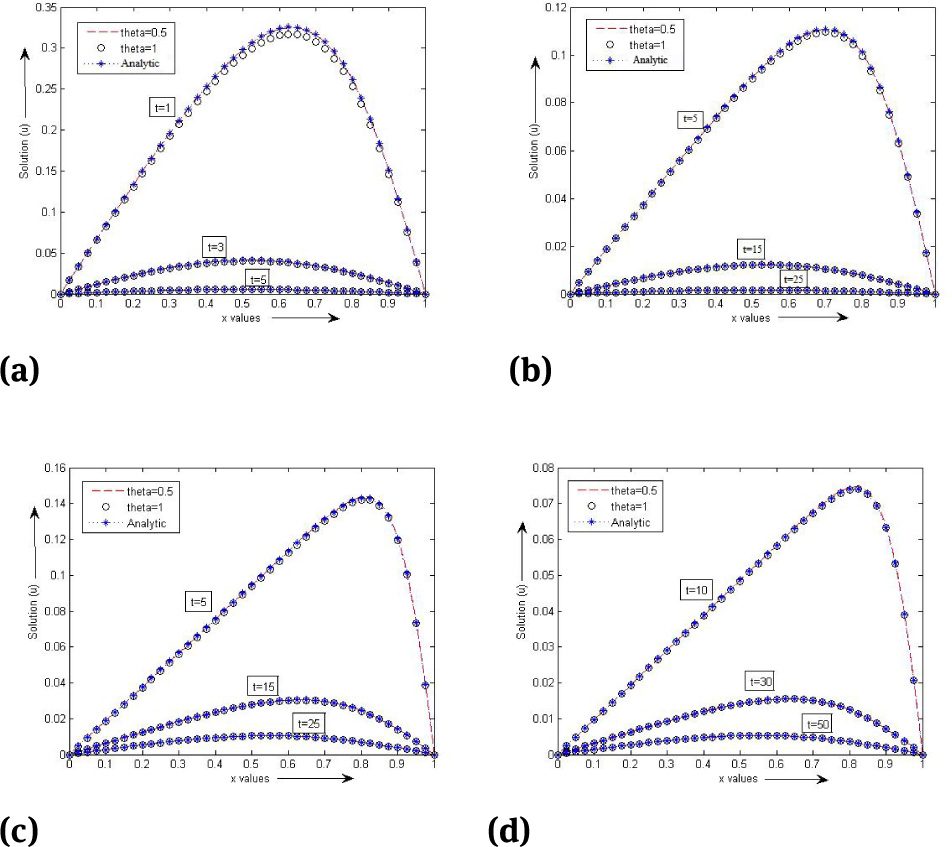
Figure 1 gives the graph of numerical solution of Example 1 for different values of v, h and Δt. In Figure 2, we have given the absolute error of our numerical method at θ = 0.5 and θ = 1. Solution profile of Example 2 is given in Figure 3 and absolute error of Example 2 for θ = 0.5 and θ = 1 is presented in Figure 4. Figures 5 and 6 respectively represent the numerical solution and the absolute error at θ = 0.5 and θ = 1 of Example 3. Figures confirm that numerical solutions are in close agreement with the analytical solution. The L2and L∞ error norms as well as the plots of absolute errors convey that θ = 0.5 (i.e. Crank-Nicolson scheme) has better accuracy than θ = 1 (i.e. backward Euler scheme)

Numerical solution of Example lat θ = 0.5 and θ = 1 at various times for space step, h=0.025 and for different values of dt and (v), (a) ν = 1, Δt = 0.0001, (b) ν = 0.1, Δt = 0.001, (c) ν = 0.02, Δt = 0.005, (d) ν = 0.01, Δt = 0.005

Absolute error of Example 1 at θ = 0.5 and θ = 1 for ν = 0.1, h = 0.0125 and Δt = 0.0001
Numerical solution of Example 2 at θ = 0.5 and θ = 1 at various times for space step, h=0.025 and for different values of Δt and(v)(a)v = l, Δt = 0.0001, (b)v = 0.1, Δt = 0.001, (c)v = 0.01, Δt = 0.005, (d)v = 0.005, Δt = 0.01

Absolute error of Example 2 at θ = 0.5 and θ = 1 for ν = 0.1, h = 0.0125 and Δt = 0.0001

Numerical solution of Example 3 at θ = 0.5 and θ = 1 at various times for space step, h=0.025 and for different values of Δt and (v)(a)v = I, Δt = 0.0001, (b)v = 0.1, Δt = 0.001, (c)v = 0.01, Δt = 0.005, (d)v = 0.005, Δt = 0.01

Absolute error of Example 3 at θ = 0.5 and θ = 1 for v = 0.005, h = 0.0125 and Δt = 0.0001
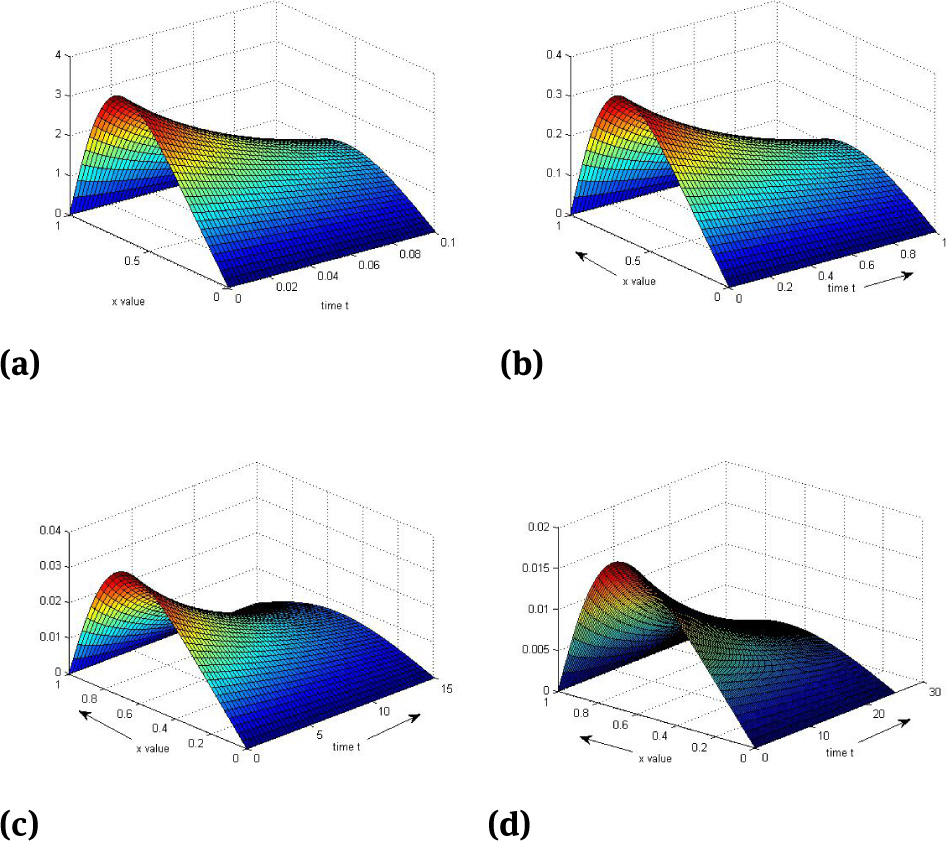
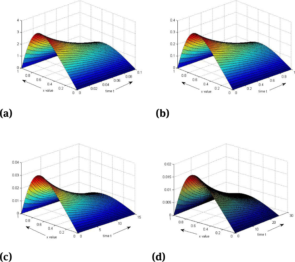
The physical behaviour of the solution of Example 1 is given in the surface plots 7 and 8. Figures 9 and 10 give the physical behaviour of the solution to Example 2. Surface plot of Example 3 is given in Figures 11 to 12. It can be seen that as time increases, the solution profile tries to attain steady state.

Surface plots of Example 1 at θ = 0.5 for space step h = 0.025 and for different values of ν and Δt, (a)v = 1, Δt = 0.002, (b)v = 0.1, Δt = 0.02, (c)v = 0.01, Δt = 0.02, (d)v = 0.005, Δt = 0.01

Surface plots of Example 1 at θ = 1 for space step h = 0.025 and for different values of ν and Δt, (a)v = l, Δt = 0.0001, (b)v = 0.1, Δt = 0.001, (c) ν = 0.01, Δt = 0.005, (d)v = 0.005, Δt = 0.01

Surface plots of Example 2 at θ = 0.5 for space step h = 0.025 and for different values of ν and∆t, (a)ν = 1,∆t = 0.001, (b)ν = 0.1, ∆t = 0.01, (c)ν = 0.01, ∆t = 0.01, (d)ν = 0.005, ∆t = 0.01

Surface plots of Example 2 at θ = 1 for space step h = 0.025 and for different values of ν and∆t, (a)ν = 1,∆t = 0.0001,(b)ν = 0.1, ∆t = 0.001, (c)ν = 0.01, ∆t = 0.005, (d)ν = 0.005, ∆t = 0.01
Surface plots of Example 3 at θ = 0.5 for space step h = 0.025 and for different values of ν and Δt, (a)v = 1, Δt = 0.002, (b)v = 0.1, Δt = 0.02, (c)v = 0.01, Δt = 0.01, (d)v = 0.005, Δt = 0.01
Surface plots of Example 3 at θ = 1 for space step h = 0.025 and for different values of ν and Δt, (a) ν = 1, Δt = 0.0001, (b) ν = 0.1, Δt = 0.001, (c)v = 0.01, Δt = 0.005, (d) ν = 0.005, Δt =0.01
7 Conclusion
Burgers’ equation is linearized by using Hopf-Cole transformation and the resultant linear Heat equation is solved by using cubic B-splines. For solving the linear Heat equation, time discretization is done using Crank-Nicolson scheme in first method and backward Euler scheme in second method. L2 and L∞error norms are computed and tabulated. The computed results are in good agreement with exact solution. The accuracy of the method is further improved by using Richardson extrapolation. It can be observed from the numerical results that Crank-Nicolson scheme is more accurate compared to backward Euler scheme. Stability analysis, which is performed using Von-Neumann stability method, proved that the proposed schemes are unconditionally stable. Comparison with the works of Kutluay et al. [1], Ozis et al. [2], Dag et al. [3], Salkuyeh et al. [4] and Korkmaz et al. [5] has validated the superiority of the proposed method over these methods. Numerical results establish that the proposed method is consistent and unconditionally stable.
References
[1] S. Kutluay, A. Esen, and I. Dag, “Numerical solution of the Burgers’ equation by the least-squares quardatic B-spline finite element method,” J· Comput. Appl. Math., vol. 167, pp. 21–33, 2004.10.1016/j.cam.2003.09.043Suche in Google Scholar
[2] T. Öziş, E. Aksan, and Α. Özdeş, “A finite element approach for solution of Burgers’ equation,” Applied Mathematics and Computation, vol. 139, no. 2, pp. 417–428, 2003.10.1016/S0096-3003(02)00204-7Suche in Google Scholar
[3] I. Dag, O. Ersoy, and O. Kacmaz, “The Trigonometric cubic B-spline algorithm for Burgers’ equation,” arXiv preprint arXiv:1407.5434, 2014.Suche in Google Scholar
[4] D. K. Salkuyeh and F. S. Sharafeh, “On the numerical solution of the Burgers’ equation,” International Journal of Computer Mathematics, vol. 86, no. 8, pp. 1334–1344, 2009.10.1080/00207160701864434Suche in Google Scholar
[5] A. Korkmaz and I. Dag, “Shock wave simulations using sinc differential quadrature method,” Engineering Computations, vol. 28, no. 6, pp. 654–674, 2011.10.1108/02644401111154619Suche in Google Scholar
[6] H. Bateman, “Some recent researches on the motion of fluids,” Monthly Weather Rev., vol. 43, pp. 163–170, 1915.10.1175/1520-0493(1915)43<163:SRROTM>2.0.CO;2Suche in Google Scholar
[7] J. M. Burgers, “Mathematical examples illustrating relations occurring in the theory of turbulent fluid motion,” Transactions on Royal Netherlands Academic Science, Amsterdam, vol. 17, pp. 1–53,1939.10.1007/978-94-011-0195-0_10Suche in Google Scholar
[8] E. Hopf, “The partial differential equation ut + uux = vuxx,” Comm. Pure Appl. Math., vol. 3, pp. 201–230,1950.10.1002/cpa.3160030302Suche in Google Scholar
[9] J. D. Cole, “On a quaslinear parabolic equations occurring in aerodynamics,” Quart. Appl. Math., vol. 9, pp. 225–236, 1951.10.1090/qam/42889Suche in Google Scholar
[10] G. Kreiss and H. O. Kreiss, “Convergence to steady state of solutions of Burgers’ equation,” Applied Numerical Mathematics, vol. 2, pp. 161–179, 1986.10.1016/0168-9274(86)90026-7Suche in Google Scholar
[11] J. Bec and K. Khanin, “Burgers’ turbulence,” Physics Reports, vol. 447, pp. 1–66, 2007.10.1016/j.physrep.2007.04.002Suche in Google Scholar
[12] E. R. Benton and G. W. Platzman, “A table of solutions of the one-dimensional Burgers’ equations,” Quart. Appl. Math., vol. 30, pp. 195–212, 1972.10.1090/qam/306736Suche in Google Scholar
[13] E. Y. Rodin, “On some approximate and exact solutions of boundary value problems for Burgers’ equation,” Journal of mathematical analysis and application, vol. 30, pp. 401–414, 1970.10.1016/0022-247X(70)90171-XSuche in Google Scholar
[14] E. Varoglu and W. D. L. Finn, “Space time finite elements incorporating characteristics for the Burgers’ equation,” Int. J. Numer. Meth. Eng., vol. 16, pp. 171–184, 1980.10.1002/nme.1620160112Suche in Google Scholar
[15] J. Caldwell, P. Wanless, and A. Cook, “A finite element approach to Burgers’ equation,” Applied Mathematical Modelling, vol. 5, no. 3, pp. 189–193, 1981.10.1016/0307-904X(81)90043-3Suche in Google Scholar
[16] J. Caldwell and P. Smith, “Solution of Burgers’ equation with a large Reynolds number,” Applied Mathematical Modelling, vol. 6, no. 5, pp. 381–385, 1982.10.1016/S0307-904X(82)80102-9Suche in Google Scholar
[17] R. Gelinas, S. Doss, and K. Miller, “The moving finite element method: applications to general Partial Differential Equations with multiple large gradients,” Journal of Computational Physics, vol. 40, no. 1, pp. 202–249, 1981.10.1016/0021-9991(81)90207-2Suche in Google Scholar
[18] J. Caldwell, P. Wanless, and A. Cook, “Solution of Burgers’ equation for large Reynolds number using finite elements with moving nodes,” Applied mathematical modelling, vol. 11, no. 3, pp. 211–214, 1987.10.1016/0307-904X(87)90005-9Suche in Google Scholar
[19] A. Dogan, “A Galerkin finite element approach to Burgers’ equation,” Applied mathematics and computation, vol. 157, no. 2, pp. 331–346, 2004.10.1016/j.amc.2003.08.037Suche in Google Scholar
[20] E. N. Aksan and A. Özdeş, “A numerical solution of Burgers’ equation,” Applied mathematics and computation, vol. 156, no. 2, pp. 395–402, 2004.10.1016/j.amc.2003.07.027Suche in Google Scholar
[21] A. Asaithambi, “Numerical solution of the Burgers’ equation by Automatic Differentiation,” Applied Mathematics and Computation, vol. 216, no. 9, pp. 2700–2708, 2010.10.1016/j.amc.2010.03.115Suche in Google Scholar
[22] M. K. Kadalbajoo, K. K. Sharma, and A. Awasthi, “A parameter-uniform implicit difference scheme for solving time-dependent Burgers’ equations,” Applied mathematics and computation, vol. 170, no. 2, pp. 1365–1393, 2005.10.1016/j.amc.2005.01.032Suche in Google Scholar
[23] Μ. Κ. Kadalbajoo and A. Awasthi, “A numerical method based on Crank-Nicolson scheme for Burgers’ equation,”Applied mathematics and computation, vol. 182, no. 2, pp. 1430–1442, 2006.10.1016/j.amc.2006.05.030Suche in Google Scholar
[24] M. Rashidi, D. Ganji, and S. Dinarvand, “Explicit analytical solutions of the generalized Burgers’ and Burger–fisher equations by homotopy perturbation method,” Numerical Methods for Partial Differential Equations, vol. 25, no. 2, pp. 409–417, 2009.10.1002/num.20350Suche in Google Scholar
[25] M. Rashidi, G. Domairry, and S. Dinarvand, “Approximate solutions for the Burgers’ and regularized long wave equations by means of the Homotopy Analysis Method,” Communications in Nonlinear Science and Numerical Simulation, vol. 14, no. 3, pp. 708–717, 2009.10.1016/j.cnsns.2007.09.015Suche in Google Scholar
[26] M. Rashidi and E. Erfani, “New analytical method for solving Burgers’ and nonlinear heat transfer equations and comparison with HAM,” Computer Physics Communications, vol. 180, no. 9, pp. 1539–1544, 2009.10.1016/j.cpc.2009.04.009Suche in Google Scholar
[27] S. Abbasbandy and M. Darvishi, “A numerical solution of Burgers’ equation by time discretization of Adomian’s Decomposition Method,” Applied mathematics and computation, vol. 170, no. 1, pp. 95–102,2005.10.1016/j.amc.2004.10.060Suche in Google Scholar
[28] S. Abbasbandy and M. Darvishi, “A numerical solution of Burgers’ equation by modified Adomian method,” Applied Mathematics and Computation, vol. 163, no. 3, pp. 1265–1272, 2005.10.1016/j.amc.2004.04.061Suche in Google Scholar
[29] M. Sarboland and A. Aminataei, “On the numerical solution of one-dimensional nonlinear nonhomogeneous Burgers’ equation,” Journal of Applied Mathematics, vol. 2014, pp. 1–15, 2014.10.1155/2014/598432Suche in Google Scholar
[30] M. Sarboland and A. Aminataei, “Taylor’s meshless petrovgalerkin method for the numerical solution of Burgers’ equation by radial basis functions,” ISRN Applied Mathematics, vol. Article ID 254086, p. 15 pages, 2012.10.5402/2012/254086Suche in Google Scholar
[31] Y. Hon and X. Mao, “An efficient numerical scheme for Burgers’ equation,” Applied Mathematics and Computation, vol. 95, no. 1, pp. 37–50, 1998.10.1016/S0096-3003(97)10060-1Suche in Google Scholar
[32] X. H. Zhang, J. Ouyang, and L. Zhang, “Element-free characteristic Galerkin method for Burgers’ equation,” Engineering Analysis with Boundary Elements, vol. 33, no. 3, pp. 356–362, 2009.10.1016/j.enganabound.2008.07.001Suche in Google Scholar
[33] V. Mukundan and A. Awasthi, “Efficient numerical techniques for Burgers’ equation,” Applied Mathematics and Computation, vol. 262, pp. 282 - 297, 2015.10.1016/j.amc.2015.03.122Suche in Google Scholar
[34] B. Inan and A. Bahadir, “An explicit exponential finite difference method for the Burgers’ equation,” European Int. J. Sci. Tech, vol. 2, pp. 61–72, 2013.Suche in Google Scholar
[35] B. Inan and A. R. Bahadir, “Numerical solution of the one-dimensional Burgers’ equation: Implicit and fully implicit exponential finite difference methods,” Pramana, vol. 81, no. 4, pp. 547–556, 2013.10.1007/s12043-013-0599-zSuche in Google Scholar
[36] B. Inan and A. R. Bahadir, “A numerical solution of the Burgers’ equation using a Crank-Nicolson exponential finite difference method,” Journal of Mathematical and Computational Science, vol. 4, no. 5, pp. 849–860, 2014.Suche in Google Scholar
[37] B. Inan and A. R. Bahadir, “Two different exponential finite difference methods for numerical solutions of the linearized Burgers’ equation,” International Journal of Modern Mathematical Sciences, vol. 13, no. 4, pp. 449–461, 2015.Suche in Google Scholar
[38] I.J. Schönberg, “Contributions to the problem of approximation of equidistant data by analytic functions,” Quart. Appl. Math, vol. 4, no. 2, pp. 45–99, 1946.10.1090/qam/15914Suche in Google Scholar
[39] H. B. Curry and I. J. Schoenberg, “On pólya frequency functions iv: the fundamental spline functions and their limits,” Journal d’analyse mathématique, vol. 17, no. 1, pp. 71–107, 1966.10.1007/BF02788653Suche in Google Scholar
[40] R. L. Roach and S. Yanping, “Unconditional stability, monotonicity and accuracy of the linear exponential interpolation function for the Burgers’ equation,” Computers & fluids, vol. 27, no. 8, pp. 963–983, 1998.10.1016/S0045-7930(98)80006-6Suche in Google Scholar
[41] A. H. A. Ali and G. A. Gardner, “A collocation solution for Burgers’ equation using cubic B-spline finite elements,” Comput. Meth.Appl. Mech. Eng., vol. 100, pp. 325–337, 1992.10.1016/0045-7825(92)90088-2Suche in Google Scholar
[42] S. Kutluay, A. Esen, and I. Dag, “Numerical solutions of the Burgers’ equation by the least-squares quadratic B-spline finite element method,” Journal of Computational and Applied Mathematics, vol. 167, no. 1, pp. 21–33, 2004.10.1016/j.cam.2003.09.043Suche in Google Scholar
[43] i. Dağ, D. Irk, and A. Şahin, “B-spline collocation methods for numerical solutions of the Burgers’ equation,” Mathematical Problems in Engineering, vol. 2005, no. 5, pp. 521–538, 2005.10.1155/MPE.2005.521Suche in Google Scholar
[44] E. Aksan, “A numerical solution of Burgers’equation by finite element method constructed on the method of discretization in time,” Applied mathematics and computation, vol. 170, no. 2, pp. 895–904, 2005.10.1016/j.amc.2004.12.027Suche in Google Scholar
[45] M.A. Ramadan, T. S. El-Danaf, and F. E. A. Alaal, “A numerical solution of the Burgers’ equation using septic B-splines,” Chaos, Solitons & Fractals, vol. 26, no. 4, pp. 1249–1258, 2005.10.1016/j.chaos.2005.02.019Suche in Google Scholar
[46] M. A. Ramadan, T. S. El-Danaf, and F. E. Alaal, “Application of the non-polynomial spline approach to the solution of the Burgers’ equation,” Open Applied Mathematics Journal, vol. 1, pp. 15–20, 2007.10.2174/1874114200701010015Suche in Google Scholar
[47] B. Saka, i. Dağ, and D. Irk, “Quintic B-spline collocation method for numerical solution of the RLW equation,” The ANZIAM Journal, vol. 49, no. 03, pp. 389–410, 2008.10.1017/S1446181108000072Suche in Google Scholar
[48] Z. Jiang and R. Wang, “An improved numerical solution of Burgers’ equation by cubic B-spline Quasi-interpolation,” J. Inform. Comput. Sci, vol. 7, no. 5, pp. 1013–1021, 2010.Suche in Google Scholar
[49] R. Mittal and P. Sighhal, “Numerical solution of Burgers’ equation,” Comm. Numer. Meth. Eng., vol. 9, pp. 397–406, 1993.10.1002/cnm.1640090505Suche in Google Scholar
[50] G. Arora and B. K. Singh, “Numerical solution of Burgers’ equation with modified cubic b-spline differential quadrature method,” Applied Mathematics and Computation, vol. 224, pp. 166–177, 2013.10.1016/j.amc.2013.08.071Suche in Google Scholar
© 2017 Walter de Gruyter GmbH, Berlin/Boston
This article is distributed under the terms of the Creative Commons Attribution Non-Commercial License, which permits unrestricted non-commercial use, distribution, and reproduction in any medium, provided the original work is properly cited.
Artikel in diesem Heft
- Frontmatter
- Nonlinear Responses and Stability of an Elastic Suspended Cable System Subjected to Parametrical External Excitations
- Modelling of imbibition phenomena in two-phase fluid flow through fractured porous media
- Application of Kudryashov and functional variable methods to the strain wave equation in microstructured solids
- Boundary layer flow of dusty fluid over a radiating stretching surface embedded in a thermally stratified porous medium in the presence of uniform heat source
- Entropy Generation with nonlinear heat and Mass transfer on MHD Boundary Layer over a Moving Surface using SLM
- Images Encryption Method using Steganographic LSB Method, AES and RSA algorithm
- Numerical simulation of Burgers’ equation using cubic B-splines