
Generalized temporal transfer matrix method: a systematic approach to solving electromagnetic wave scattering in temporally stratified structures
-
Jingwei Xu

 ,
Wending Mai
and
Douglas H. Werner
,
Wending Mai
and
Douglas H. Werner

Abstract
Opening a new door to tailoring electromagnetic (EM) waves, temporal boundaries have attracted the attention of researchers in recent years, which have led to many intriguing applications. However, the current theoretical approaches are far from enough to handle the complicated temporal systems. In this paper, we develop universal matrix formalism, paired with a unique coordinate transformation technique. The approach can effectively deal with temporally stratified structures with complicated material anisotropy and arbitrary incidence angles. This formulation is applied to various practical systems, enabling the solution of these temporal boundary related problems in a simple and elegant fashion, and also facilitating a deep insight into the fundamental physics.
1 Introduction
Time-varying metamaterials and metasurfaces facilitate a new degree of freedom for controlling electromagnetic (EM) waves. In recent years, significant efforts have been devoted to this topic, enabling some novel phenomena such as non-reciprocity, frequency conversion [1], [2], [3], [4], [5], dispersion engineering [6], asymmetric propagation [7], bandwidth extension [8], harmonic information transition [9], time-varying optical vortices [10], and spectrum spreading [11]. These characteristics typically can’t be achieved with conventional metamaterials and metasurfaces that are time-invariant and designed to operate in the frequency domain. Active components are usually required in order to bestow metasurfaces with the desired time-modulation, such as lumped elements [1], real-time interference patterns [2], and optical pumping [3].
Despite the significant achievements made by researchers, the time modulation is usually confined to a small volume (i.e., within metasurface unit cells), and consequently the desired phenomena, such as frequency conversion or harmonic transition, are still characterized in the time-invariant regime. One may be naturally curious, however, regarding what would happen if the time modulation were to occur over a much larger region. In [12], the authors proposed the revolutionary concept of a temporal boundary. Their work describes an EM wave propagating in an infinite homogeneous medium (see Figure 1a), whose material parameters
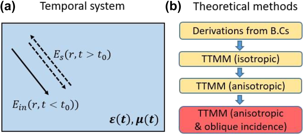
(a) Schematics of temporal boundary value problems (TBVPs). (b) Flowchart showing the current theoretical approaches for the system described in (a) where the contribution of this paper is highlighted in red.
Having been explored theoretically and numerically, this concept soon mushroomed into a rich topic of research over the past several years. Many concepts have emerged that rely on tailoring waves at spatial boundaries and transforming them to the temporal domain. They include effective medium theory [13, 14], anti-reflection coatings [15], Fabry–Perot cavities [16, 17], prisms [18], waveguides [19, 20], photonic crystals [21], [22], [23], polarization conversion [24], total internal reflection [25], the Brewster angle [26], parity-time (PT) symmetry [27], and impedance transformers [28]. Moreover, by utilizing temporal boundaries, some ideas unique to temporal systems have also been explored. For example, in [29], the authors were able to achieve a real-time redirection of energy propagation. The notion of EM cloaks was generalized in [30], so that an ‘event’, rather than an object, could be concealed. In [31], it was found that there is an exponential increase of intensity when a wave travels through a temporally disordered structure. The energy conservation issue associated with a pulse travelling through a temporal boundary is investigated in [32]. Finally, in [33, 34], the authors studied the properties of temporal discontinuities in dispersive media. These concepts and associated designs result from solving the appropriate Temporal Boundary Value Problem (TBVP): a terminology which we adopt in our later discussions.
While these applications bring new opportunities in optics and electromagnetics, many of them involve complex temporal systems, including multiple (or even infinite) temporal boundaries [13], [14], [15], [16, 21], [22], [23], [24, 28] and anisotropic materials [18, 24, 26, 29]. Thus, the formulation introduced in [12], which is targeted to an EM wave’s reflection and transmission near a single temporal boundary, while revolutionary, is quite limited in terms of its applicability to solving more general TBVPs. Much of the literature [13, 15, 16, 18, 26, 29] relies on direct derivations from the boundary conditions of Maxwell’s equations in order to calculate the desired quantities, such as S parameters. In fact, all of the derivations are based on the same principle; consequently, they are inevitably repetitive, and sometimes lengthy. In some cases considered in the literature [22, 31], the temporal systems are too complex to have a closed form solution. Therefore, the important question arises; can an overarching theoretical approach be developed to handle all the TBVPs?
Indeed, there are some theoretical works that have attempted to address EM wave propagation inside materials with arbitrary
In light of this shortcoming, in this paper, we introduce a theoretical framework that can handle EM wave interactions with homogenous time-variant materials, for arbitrary incident angles, and material anisotropy. First, we demonstrate that the concept of ‘oblique incidence’ needs to be clarified and re-defined, which poses a challenge in solving problems with temporal boundaries. Then, we adopt a coordinate transformation strategy in order to address this issue, and develop a method that we call generalized TTMM (GTTMM). Using this method, we successfully analyze EM wave responses in several practical temporal systems. Moreover, numerical simulations are also performed to validate the analytical results.
2 Challenges
First, we revisit the conventional
Hence, in this formalism, the transfer matrix needs to have a dimension of four in order to fully describe the properties of the EM system. Equation (1) is valid no matter whether the wave is obliquely or normally incident, because the normal to the interface is always along the
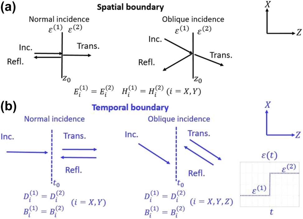
Schematics showing the difference between (a) spatial and (b) temporal boundaries, in terms of the associated boundary conditions.
Now let us consider a temporal scenario such that the wave is travelling in a homogeneous material, which changes suddenly from medium 1 to 2 (see Figure 2b). In this case, however, the boundary conditions of Maxwell’s equations require that all three components of the
Here, there are six independent equations which must be solved simultaneously. Obviously, the classical
With this assumption, the formalism presented in [40] could be easily adapted to produce a temporal counterpart, because the number of independent equations is reduced to 4. However, what happens if the wave does not propagate in
In order to address this dilemma, we resort to a ‘coordinate transformation technique’. Specifically, the anisotropy of the material and the incident wave define two coordinate systems:
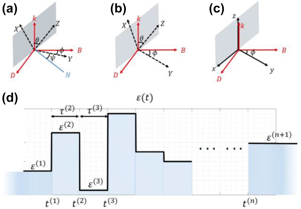
(a)–(c) Schematics illustrating the coordinate transformation. (a) The Euler angle representation of S1 and S2.
At this point, for simplicity, a special case:
3 Theoretical formulation
3.1 TTMM formalism
Before establishing the TTMM formalism, let us define the temporal system (Figure 3d). It consists of an unbounded homogenous medium, whose permittivity or permeability undergoes abrupt changes
Several assumptions are made about the system: (a) The anisotropy of each temporal layer shares the same principal axes (
where
where
Notice that
where
Similar to the discussions in [24, 40], one can express the
where {
By applying the boundary conditions at the
we have
where
and
Importantly, at this point in the development, it is not clear what role the incidence angle would play in a generalized formulation. In the following section, however, we will see that when the wave is obliquely incident (i.e., S1 and S3 do not overlap), the relation between
3.2 Explicit form of the transfer matrices
First, let us investigate the dispersion relation, as determined by Eq. (5). For each temporal layer, we replace
where
These quantities can be viewed as the equivalent refractive indices seen by x- and y-polarized waves inside the
It then follows that the corresponding field vectors of
Clearly, these four solutions correspond to the two orthogonal modes (i.e., y- and x-polarized waves) propagating in opposite directions. Next, we use Eqs. (6.2), (10) and (11.4) to obtain:
which can be rewritten as:
At this point we define the following identities:
which can be viewed as the equivalent impedances seen by the x- and y-polarized waves inside the
With the explicit form of matrices
From the discussion above, we know that the
At this point we have completed our introduction to the GTTMM. In the next two sections, we will apply this tool to four different temporal systems, which are schematically represented in Figure 4. All of these systems can be regarded as temporal multilayer structures, as have been described in Figure 3d. Moreover, the desired physical quantities, for example, the permittivity tensor of the anisotropic antireflection temporal coating or the transmission coefficients in the case of polarization conversion, could be calculated directly from the
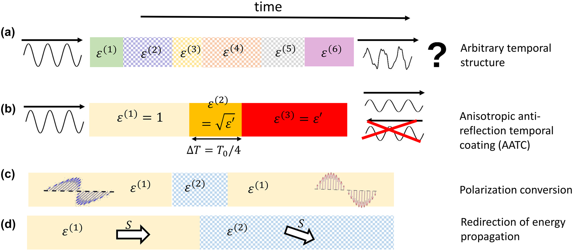
Schematics of several temporal systems.
The different temporal regions are represented by colored boxes. The temporal profile in the case of (a) an arbitrary temporal structure, (b) an anisotropic antireflection temporal coating, (c) polarization conversion, and (d) redirection of energy propagation. Notice that anisotropic temporal regions are denoted by checkerboard patterns.
4 Application: anisotropic systems
In this section, we will consider some practical TBVPs to demonstrate the application and efficacy of the GTTMM. These TBVPs are relatively complicated, involving multilayer anisotropic temporal structures, which are later simply referred to as ‘structure(s)’. First, in Section A, we introduce a 6-layer structure with a random profile and use it to demonstrate the robustness of our method. Next, in Section 4B, we generalize the idea of an antireflection temporal coating (ATC) [15] to the anisotropic case. In [24], we found that the polarization state of a wave would experience a temporal change if an ‘anisotropic temporal slab’ is ‘inserted’ into an isotropic background medium. Researchers in [25] temporally switched the material permittivity from isotropic to anisotropic, and found that the Poynting vector (i.e., energy flux) of the wave will change in time. Referring to the coordinates illustrated in Figure 3b, the case where
For all four examples studied here, we present comparisons of the results obtained from the GTTMM calculations and FDTD simulations. Apart from these examples, we also show that the GTTMM formulation can be reduced to the isotropic scenario as a special case. For verification, we re-derived the results presented in two previously published papers using the GTTMM (see Supplemental Document 2).
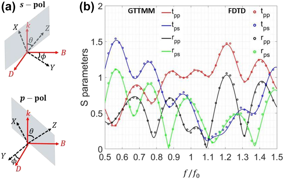
An arbitrary temporal structure: (a) the coordinate representation of two polarization states in the S2 system, where the grey parallelograms denote the XZ plane. (b) S parameters, where the GTTMM and FDTD results are represented by solid lines and dots, respectively.
4.1 Arbitrary multi-layer temporal structure
First, in order to demonstrate the validity of our GTTMM algorithm, we consider a 6-layer structure, which has a random profile. The information on the composition of this structure is displayed in Table 1. Notice that the first and last layers are isotropic, and they are semi-infinite in time. Now, let us study the interactions between the electromagnetic waves and this structure. As mentioned before, two independent parameters,
Profile of the arbitrary 6-layer temporal structure. The first and the last (i.e., the 6th) layers are isotropic materials. The duration of each layer is normalized to
| Layer | 1 | 2 | 3 | 4 | 5 | 6 |
|---|---|---|---|---|---|---|
|
|
1 | 4 | 8 | 12 | 2 | 1 |
|
|
13 | 9 | 5 | 6 | ||
|
|
2 | 7 | 3 | 10 | ||
|
|
NA | 1.35 | 2.22 | 1.27 | 1.74 | NA |
Figure 5 shows the spectral response of a
4.2 Polarization conversion
Polarization conversion is an important property with many practical applications in optics and electromagnetics. Traditionally, one could convert polarization of an EM wave by utilizing the interface between an isotropic and an anisotropic material [43]. In our previous work [24], we extended this idea to the temporal domain, and achieved complete polarization conversions in real time, as schematically demonstrated in Figure 4c. In that work, however, we only considered the normal incidence case (
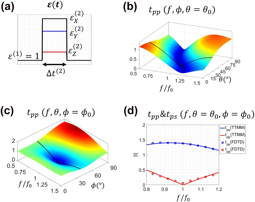
Illustrations of the polarization conversion effect. (a) Schematic of the temporal profile of the system (b)–(d) the transmission spectra.
After some mathematical manipulations, we arrive at the following result:
for which
where
CPC means that the incident wave is completely converted to the orthogonal polarization for certain values of
4.3 Anisotropic antireflection temporal coating (AATC)
V. Pacheco-Pena et al. recently introduced the intriguing concept of an antireflection temporal coating (ATC) in the time domain [15]. We know from the theory of temporal boundaries that there is a reflection when the material permittivity undergoes a sudden change (e.g., from
where
In [15], however, the authors only consider the case where the material is isotropic. One may be naturally curious as to what conditions the material properties should satisfy in order to minimize reflection if anisotropic materials are involved. In other words, is it possible to derive a similar expression to Eq. (18) using the GTTMM?
To be more specific, we consider the following temporal structure comprising of three temporal regions, whose permittivities are
where the definition of
Next, for a practical illustration, we arbitrarily choose a combination of parameters that satisfy Eq. (19):
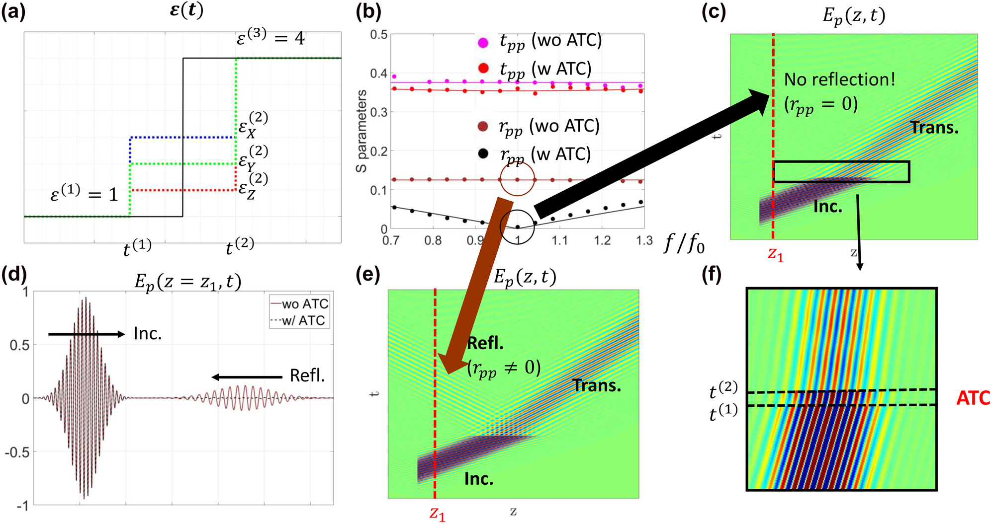
Illustration of an anisotropic anti-reflection temporal coating (AATC).
(a) The temporal profiles with and without the AATC. (b) Transmission and reflection spectra with and without the AATC, where the GTTMM and FDTD results are represented by solid lines and dots, respectively. (c) and (e) FDTD simulation results of
Similar to the approach adopted in Section 4A, we have plotted the spectral response of a
As a comparison, we consider another case where
This example represents a natural but highly nontrivial generalization of the work reported in [15]. By comparing with the work in [15], our presented results cannot be easily understood from a space-time symmetry perspective. Rather, a rigorous GTTMM analysis is required to derive the conditions for reflection cancellation.
4.4 Redirection of energy flow
One of the interesting features of temporal boundaries is that the

Demonstrations of the redirection of energy propagation.
(a) The temporal profile of the system. (b)
Next, let us calculate the value of
where
After simplification (see Supplemental Document 3), we have
Clearly,
Now, we consider a specific material profile:
5 Conclusions
In this paper, we proposed a rigorous analytical methodology, which we call GTTMM, to evaluate wave propagation in temporally stratified structures, based on the application of the appropriate boundary conditions to Maxwell’s equations. Then we applied this theory to several temporal systems, and confirmed its validity using full-wave FDTD simulations. These studies targeted anisotropic material systems, which have important applications but are typically difficult to solve due to their relatively complex mathematical descriptions. Comparing with the traditional methods presented in [13, 15, 16, 18, 29], our approach is more elegant as well as concise. With this tool, we can tackle more complicated problems; all four TBVPs we considered represent generalizations of previously studied system. More importantly, it is universal and can be applied as a powerful tool for solving a very broad class of TBVPs. From antireflection coatings to polarizers, we have shown that these completely different applications can be considered as part of the same overarching theoretical framework. In addition to the effectiveness demonstrated in solving these problems, this framework also reveals some rich insights into the fundamental physics. First, it reveals the mathematical similarities between all these seemingly different systems. Besides, it sheds light on the unique properties of temporal boundaries and has prompted us to reconsider some well-established concepts such as oblique incidence. In conclusion, our formalism represents a powerful tool for solving TBVPs. Moreover, it is expected to serve an important role in the future design of potentially transformative devices, as the current temporal modulation techniques continue to grow more mature.
-
Author contribution: All the authors have accepted responsibility for the entire content of this submitted manuscript and approved submission.
-
Research funding: This research was supported in part by DARPA EXTREME (contract HR00111720032).
-
Conflict of interest statement: The authors declare no conflicts of interest regarding this article.
References
[1] L. Zhang, X. Q. Chen, R. W. Shao, et al.., “Breaking reciprocity with space-time-coding digital metasurfaces,” Adv. Mater., vol. 31, p. 1904069, 2019. https://doi.org/10.1002/adma.201904069.Search in Google Scholar PubMed
[2] X. Guo, Y. Ding, Y. Duan, and X. Ni, “Nonreciprocal metasurface with space–time phase modulation,” Light Sci. Appl., vol. 8, p. 123, 2019. https://doi.org/10.1038/s41377-019-0225-z.Search in Google Scholar PubMed PubMed Central
[3] Y. Zhou, M. Z. Alam, M. Karimi, et al.., “Broadband frequency translation through time refraction in an epsilon-near-zero material,” Nat. Commun., vol. 11, p. 2180, 2020. https://doi.org/10.1038/s41467-020-15682-2.Search in Google Scholar PubMed PubMed Central
[4] S. Taravati and G. V. Eleftheriades, “Pure and Linear Frequency Converter Temporal Metasurface,” ArXiv210303360 Phys. 2021.10.21203/rs.3.rs-241598/v1Search in Google Scholar
[5] X. Wang, G. Ptitcyn, A. Díaz-Rubio, et al.., “Nonreciprocity in bianisotropic systems with uniform time modulation,” ArXiv200102213 Phys. 2020, https://doi.org/10.1103/physrevlett.125.266102.Search in Google Scholar PubMed
[6] N. Chamanara, Z.-L. Deck-Léger, C. Caloz, and D. Kalluri, “Unusual electromagnetic modes in space-time-modulated dispersion-engineered media,” Phys. Rev. A, vol. 97, 2018, Art no. 063829. https://doi.org/10.1103/physreva.97.063829.Search in Google Scholar
[7] P. Biswas, H. K. Gandhi, and S. Ghosh, “Asymmetric propagation and limited wavelength translation of optical pulses through a linear dispersive time-dynamic system,” Opt. Lett., vol. 44, p. 3022, 2019. https://doi.org/10.1364/ol.44.003022.Search in Google Scholar PubMed
[8] H. Li and A. Alù, “Temporal switching to extend the bandwidth of thin absorbers,” Optica, vol. 8, p. 24, 2021. https://doi.org/10.1364/optica.408399.Search in Google Scholar
[9] H. Wu, X. X. Gao, L. Zhang, et al.., “Harmonic information transitions of spatiotemporal metasurfaces,” Light Sci. Appl., vol. 9, p. 198, 2020. https://doi.org/10.1038/s41377-020-00441-1.Search in Google Scholar PubMed PubMed Central
[10] H. Barati Sedeh, M. M. Salary, and H. Mosallaei, “Time-varying optical vortices enabled by time-modulated metasurfaces,” Nanophotonics, vol. 9, p. 2957, 2020. https://doi.org/10.1515/nanoph-2020-0202.Search in Google Scholar
[11] X. Wang and C. Caloz, “Spread-spectrum selective camouflaging based on time-modulated metasurface,” ArXiv190904480 Phys. 2019.10.1109/APUSNCURSINRSM.2019.8888333Search in Google Scholar
[12] Y. Xiao, D. N. Maywar, and G. P. Agrawal, “Reflection and transmission of electromagnetic waves at a temporal boundary,” Opt. Lett., vol. 39, p. 574, 2014. https://doi.org/10.1364/ol.39.000574.Search in Google Scholar PubMed
[13] V. Pacheco-Peña and N. Engheta, “Effective medium concept in temporal metamaterials,” Nanophotonics, vol. 9, p. 379, 2020.10.1515/nanoph-2019-0305Search in Google Scholar
[14] V. Pacheco-Peña and N. Engheta, “Temporal metamaterials with gain and loss,” ArXiv210801007 Phys. 2021.Search in Google Scholar
[15] V. Pacheco-Peña and N. Engheta, “Antireflection temporal coatings,” Optica, vol. 7, p. 323, 2020.10.1364/OPTICA.381175Search in Google Scholar
[16] D. Ramaccia, A. Toscano, and F. Bilotti, “Light propagation through metamaterial temporal slabs: reflection, refraction, and special cases,” Opt. Lett., vol. 45, p. 5836, 2020. https://doi.org/10.1364/ol.402856.Search in Google Scholar PubMed
[17] J. Zhang, W. R. Donaldson, and G. P. Agrawal, “Time-domain fabry–perot resonators formed inside a dispersive medium,” J. Opt. Soc. Am. B, vol. 38, p. 2376, 2021. https://doi.org/10.1364/josab.428411.Search in Google Scholar
[18] A. Akbarzadeh, N. Chamanara, and C. Caloz, “Inverse prism based on temporal discontinuity and spatial dispersion,” Opt. Lett., vol. 43, p. 3297, 2018. https://doi.org/10.1364/ol.43.003297.Search in Google Scholar
[19] B. W. Plansinis, W. R. Donaldson, and G. P. Agrawal, “Temporal waveguides for optical pulses,” J. Opt. Soc. Am. B, vol. 33, p. 1112, 2016. https://doi.org/10.1364/josab.33.001112.Search in Google Scholar
[20] J. Zhou, G. Zheng, and J. Wu, “Comprehensive study on the concept of temporal optical waveguides,” Phys. Rev. A, vol. 93, 2016, Art no. 063847. https://doi.org/10.1103/physreva.93.063847.Search in Google Scholar
[21] E. Lustig, Y. Sharabi, and M. Segev, “Topological aspects of photonic time crystals,” Optica, vol. 5, p. 1390, 2018. https://doi.org/10.1364/optica.5.001390.Search in Google Scholar
[22] Y. Sharabi, E. Lustig, and M. Segev, “Disordered photonic time crystals,” Phys. Rev. Lett., vol. 126, p. 163902, 2021. https://doi.org/10.1103/physrevlett.126.163902.Search in Google Scholar PubMed
[23] J. S. Martínez-Romero, O. M. Becerra-Fuentes, and P. Halevi, “Temporal photonic crystals with modulations of both permittivity and permeability,” Phys. Rev. A, vol. 93, 2016, Art no. 063813.10.1103/PhysRevA.93.063813Search in Google Scholar
[24] J. Xu, W. Mai, and D. H. Werner, “Complete polarization conversion using anisotropic temporal slabs,” Opt. Lett., vol. 46, p. 1373, 2021. https://doi.org/10.1364/ol.415757.Search in Google Scholar PubMed
[25] B. W. Plansinis, W. R. Donaldson, and G. P. Agrawal, “What is the temporal analog of reflection and refraction of optical beams?” Phys. Rev. Lett., vol. 115, p. 183901, 2015. https://doi.org/10.1103/physrevlett.115.183901.Search in Google Scholar PubMed
[26] V. Pacheco-Peña and N. Engheta, “Temporal brewster angle,” ArXiv210213305 Phys. 2021.Search in Google Scholar
[27] H. Li, S. Yin, E. Galiffi, and A. Alù, “Temporal parity-time symmetry for extreme energy transformations,” Phys. Rev. Lett., vol. 127, p. 153903, 2021. https://doi.org/10.1103/physrevlett.127.153903.Search in Google Scholar
[28] G. Castaldi, V. Pacheco-Peña, M. Moccia, N. Engheta, and V. Galdi, “Exploiting space-time duality in the synthesis of impedance transformers via temporal metamaterials,” Nanophotonics, vol. 0, 2021, Art no. 000010151520210231. https://doi.org/10.1515/nanoph-2021-0231.Search in Google Scholar
[29] V. Pacheco-Peña and N. Engheta, “Temporal aiming,” Light Sci. Appl., vol. 9, p. 129, 2020.10.1038/s41377-020-00360-1Search in Google Scholar PubMed PubMed Central
[30] M. W. McCall, A. Favaro, P. Kinsler, and A. Boardman, “A spacetime cloak, or a history editor,” J. Opt., vol. 13, 2011, Art no. 029501. https://doi.org/10.1088/2040-8978/13/2/029501.Search in Google Scholar
[31] Y. Sharabi, E. Lustig, and M. Segev, “Light propagation in temporally disordered media,” in Conference on Lasers and Electro-Optics, San Jose, California, OSA, 2019, p. FF3B.1.10.1364/CLEO_QELS.2019.FF3B.1Search in Google Scholar
[32] K. B. Tan, H. M. Lu, and W. C. Zuo, “Energy conservation at an optical temporal boundary,” Opt. Lett., vol. 45, p. 6366, 2020. https://doi.org/10.1364/ol.405310.Search in Google Scholar
[33] M. I. Bakunov, A. V. Shirokova, M. A. Kurnikov, and A. V. Maslov, “Light scattering at a temporal boundary in a lorentz medium,” Opt. Lett., vol. 46, p. 4988, 2021. https://doi.org/10.1364/ol.437419.Search in Google Scholar
[34] D. M. Solís, R. Kastner, and N. Engheta, “Time-varying materials in the presence of dispersion: plane-wave propagation in a lorentzian medium with temporal discontinuity,” Photon. Res., vol. 9, p. 1842, 2021.10.1364/PRJ.427368Search in Google Scholar
[35] T. T. Koutserimpas and R. Fleury, “Electromagnetic fields in a time-varying medium: exceptional points and operator symmetries,” IEEE Trans. Antenn. Propag., vol. 68, no. 9, pp. 6717–6724, 2020. https://doi.org/10.1109/tap.2020.2996822.Search in Google Scholar
[36] M. Chegnizadeh, K. Mehrany, and M. Memarian, “General solution to wave propagation in media undergoing arbitrary transient or periodic temporal variations of permittivity,” J. Opt. Soc. Am. B, vol. 35, p. 2923, 2018. https://doi.org/10.1364/josab.35.002923.Search in Google Scholar
[37] M. Born and E. Wolf, Principles of Optics: Electromagnetic Theory of Propagation, Interference and Diffraction of Light, Oxford, Pergamon, 1980.Search in Google Scholar
[38] D. Ramaccia, A. Alù, A. Toscano, and F. Bilotti, “Temporal multilayer structures for designing higher-order transfer functions using time-varying metamaterials,” Appl. Phys. Lett., vol. 118, p. 101901, 2021. https://doi.org/10.1063/5.0042567.Search in Google Scholar
[39] J. Zhang, W. R. Donaldson, and G. P. Agrawal, “Impact of the boundary’s sharpness on temporal reflection in dispersive media,” Opt. Lett., vol. 46, p. 4053, 2021. https://doi.org/10.1364/ol.432180.Search in Google Scholar PubMed
[40] J. Hao and L. Zhou, “Electromagnetic wave scatterings by anisotropic metamaterials: generalized 4 × 4 transfer-matrix method,” Phys. Rev. B, vol. 77, 2008, Art no. 094201. https://doi.org/10.1103/physrevb.77.094201.Search in Google Scholar
[41] V. Pacheco-Peña and N. Engheta, “Spatiotemporal isotropic- to-anisotropic meta-atoms,” New J. Phys., vol. 23, 2021, Art no. 095006.10.1088/1367-2630/ac21dfSearch in Google Scholar
[42] H. Goldstein, Classical Mechanics, 2nd ed., Reading, Mass, Addison-Wesley Pub. Co, 1980.Search in Google Scholar
[43] J. Hao, Y. Yuan, L. Ran, et al.., “Manipulating electromagnetic wave polarizations by anisotropic metamaterials,” Phys. Rev. Lett., vol. 99, 2007, Art no. 063908. https://doi.org/10.1103/PhysRevLett.99.063908.Search in Google Scholar PubMed
Supplementary Material
The online version of this article offers supplementary material (https://doi.org/10.1515/nanoph-2021-0715).
© 2022 Jingwei Xu et al., published by De Gruyter, Berlin/Boston
This work is licensed under the Creative Commons Attribution 4.0 International License.
Articles in the same Issue
- Frontmatter
- Reviews
- Gaptronics: multilevel photonics applications spanning zero-nanometer limits
- Ultrafast photonics applications of emerging 2D-Xenes beyond graphene
- Research Articles
- Nonlocal effects in temporal metamaterials
- Pattern-tunable synthetic gauge fields in topological photonic graphene
- Generalized temporal transfer matrix method: a systematic approach to solving electromagnetic wave scattering in temporally stratified structures
- Femtosecond imaging of spatial deformation of surface plasmon polariton wave packet during resonant interaction with nanocavity
- Probing the long-lived photo-generated charge carriers in transition metal dichalcogenides by time-resolved microwave photoconductivity
- Second-order topological phases in C 4v -symmetric photonic crystals beyond the two-dimensional Su-Schrieffer–Heeger model
- Full-visible-spectrum perovskite quantum dots by anion exchange resin assisted synthesis
- Multidimensional engineered metasurface for ultrafast terahertz switching at frequency-agile channels
- High efficiency and large optical anisotropy in the high-order nonlinear processes of 2D perovskite nanosheets
- Dynamic millimeter-wave OAM beam generation through programmable metasurface
- Intelligent metasurface with frequency recognition for adaptive manipulation of electromagnetic wave
- Singularities splitting phenomenon for the superposition of hybrid orders structured lights and the corresponding interference discrimination method
- Inverse-designed waveguide-based biosensor for high-sensitivity, single-frequency detection of biomolecules