Novel weighted distribution: Properties, applications and web-tool
-
Emrah Altun
 und
Christophe Chesneau
und
Christophe Chesneau

Abstract
Weighted distributions play an important role in reliability and engineering. This research contributes to the topic by presenting a novel flexible two-parameter weighted distribution characterized by extensive statistical properties. Various parameter estimation methods are also thoroughly investigated. Their effectiveness is validated by complete simulation studies. Within the framework of generalized linear models, a regression model is established for positively defined response variables. Two data sets are examined to emphasize the importance of the proposed model. In addition, the WBreg tool is presented to facilitate its use by researchers. WBreg is available “free of charge” at https://beststat.shinyapps.io/WB2reg.
1 Introduction
Weighted distributions play an important role in several applied fields, including ecology, reliability and biology. In [20], weighted distributions to human populations and wildlife management were applied. In [17], the importance of weighted distributions in reliability and life testing was studied. In [19], the utility of weighted distributions in ecology, particularly in the context of resource selection probabilities, was demonstrated. The general definition of a weighted distribution is based on a probability density function (pdf) of the following form:
where D is the normalization constant, w(x) is the weighting function and f(x) is a given pdf, usually from a known baseline distribution. Note that when w (x) = x, the resulting distribution is called a length-biased distribution [15]. Several weighted distributions have been proposed using the mathematical equation in (1.1), such as the weighted Lomax distribution by [3], the weighted Lindley distribution by [15], the weighted gamma distribution by [18], the weighted Weibull distribution by [12], and the weighted xgamma distribution by [23].
For the purposes of this research, we need to introduce a remarkable distribution known as the Bilal (B) distribution. First proposed by [1], it has emerged as a direct competitor to the exponential and Lindley distributions. Since then, the B distribution has received a lot of attention from researchers. [7] introduced the log-Bilal distribution and developed its regression model for bounded response variables in the interval (0, 1). [8] obtained a new one-parameter discrete distribution derived from the B distribution. [6] introduced a new mixed Poisson distribution by using the B distribution as a mixture distribution. A generalization of the B distribution was proposed by [2]. [22] introduced the power B distribution and applied it to some COVID-19 data. This literature review shows that the B distribution has been extensively studied by researchers and remains of modern interest.
In this research, we introduce the weighted Bilal (WB) distribution following the results of [15]. A size-biased version of the B distribution has been studied by [5]. Their work introduces an order value, t, which is taken to be a fixed value. More precisely, [5] studied the special cases of the size-biased B distribution, such as the length-biased B distribution for t = 1 and the area-biased B distribution for t = 2. The resulting distributions thus have one parameter. However, we believe that significant flexibility can be gained by considering the parameter t as a variable. We therefore consider a one-parameter weighting function to obtain a more flexible distribution. The proposed WB distribution has a simple form and tractable properties. We study its mathematical properties in detail. The parameter estimation process is carried out using three approaches, and simulation studies are given for each approach. The WB regression model is defined using the generalized linear models approach. The parameter estimation process and residual analysis of the WB regression model are also discussed. The model is tested on life expectancy data and the results are interpreted. In addition, a cloud-based software called WBreg is developed in the R Shiny environment. The aim is to ensure widespread use of the model developed.
The research is organized as follows: The second section provides an in-depth examination of the statistical properties associated with the WB model. The third section outlines the various methods employed for parameter estimation. The fourth section compares these techniques with the results of a simulation study. Section five defines a new regression model based on the WB model, discussing both parameter estimation and residual analysis for this model. Section six presents two applications and introduces WBreg, the software developed for the WB model. The seventh section concludes by summarizing the main findings of the research.
2 Weighted Bilal distribution
2.1 Presentation
We start with the presentation of the WB distribution, which leads to a recall on the B distribution. The pdf and cumulative distribution function (cdf) of the B distribution are, respectively,
where x > 0 and θ > 0. Using the idea of [15], we propose the WB distribution with one extra shape parameter. It is therefore defined as
where f0(x; θ) is the pdf of the B distribution in (2.1), C refers to the normalization constant, and α > 0. Using the definition in (2.3) and after computing C, the pdf of the WB distribution is
where x > 0, θ > 0, α > 0 and Γ (·) is the standard gamma function. After integrating this pdf, the cdf of the WB distribution is as follows:
where
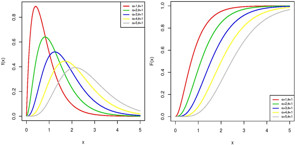
The pdf and cdf plots of the WB distribution.
2.2 Properties
Some of the properties of the WB distribution can be derived from the work in [5]. In this subsection, we only highlight or develop those that are determinant or new.
Important functions are the survival and hazard rate functions of the WB distribution, given, respectively, by
The behaviour of the pdf at x = 0 and x → ∞ can be investigated. When x → ∞, by the decreasingness properties of the exponential function that dominate the power weighting function, we get f (x) → 0. When x → 0, since
and α > 0, we have f (x) → 0.
As a new structural remark, the pdf of the WB distribution can be re-defined as follows:
We recognize a mixture representation of two pdfs associated with the standard gamma distribution, that is
where w = 3α/(3α – 2α), f1(x; α, θ) and f2(x; α, θ) are the pdfs associated with the distributions Gamma(shape = α, scale = θ/2) and Gamma (shape = α, scale = θ/3). Obviously, most of the statistical properties of the WB distribution can be obtained using the mixture representation.
The proposition below deals with the expression of the raw moments associated with the WB distribution.
Proposition 1
The rth raw moment of a random variable X with the WB distribution is
For ease of reading, the proof of this proposition and the results to be obtained are postponed to the appendix.
Thanks to Proposition 1, the mean and variance associated with the WB distribution are
In a sense, the proposition below completes Proposition 1; it determines the moment generating function associated with the WB distribution.
Proposition 2
The moment generating function associated with the WB distribution is
Similarly, the characteristic function associated with the WB distribution is given in the proposition below.
Proposition 3
The characteristic function associated with the WB distribution is
To conclude this analysis, we present the mode of the WB distribution for the case α ≥ 1.
Proposition 4
For α ≥ 1, the mode of the WB distribution is given by
3 Estimation
We now develop the parametric estimation in the context of the WB distribution, namely, the maximum likelihood estimation (MLE), the least squares estimation (LSE) and the weighted LSE (WLSE).
3.1 Maximum likelihood
Assume that x1, x2, . . . , xn is a random sample from the WB distribution. In the setting of the MLE, based on the pdf in (2.4), the associated log-likelihood function is
where
where
where
where
where zp/2 denotes the %p/2 quantile value derived from the standard normal distribution, N (0, 1). This quantile can be readily obtained using the quantile function associated with this normal distribution.
The study has two significant limitations. First, since the parameter estimates cannot be obtained in closed form, it takes a long time to compute large data sets. The second is that, when there are a large number of outliers in the data set, the parameter estimates can be biased and yield high standard errors. Therefore, robust parameter estimation methods need to be employed. This is planned for future work.
3.2 Other estimation methods
We now consider the order values of x1, x2, . . . , xn, denoted as x1:n, x2:n, . . . , xn:n. The derivation of LSEs and WLSEs is achieved through the minimization of the following functions:
4 Simulation study
In this section, the MLE, LSE and WLSE methods are compared through a simulation study. Two parameter vectors are used. These are α = 0.5, θ = 2 and α = 2, θ = 5. The simulation is repeated by 1000 times. Three sample sizes are used. These are n = 50, 100 and 500. The bias and mean squared error (MSE) are calculated using estimated parameter values and theirs true values. The results are summarized in Table 1. We have the following results:
Comparison of estimation methods.
| Parameters | Sample sizes | Metrics | MLE |
LSE |
WLSE |
|||
|---|---|---|---|---|---|---|---|---|
| α | θ | α | θ | α | θ | |||
| α = 0:5 | 50 | Bias | 0.084 | –0.029 | 0.044 | 0.105 | 0.049 | 0.064 |
| MSE | 0.108 | 0.192 | 0.154 | 0.333 | 0.133 | 0.263 | ||
| 100 | Bias | 0.046 | –0.028 | 0.020 | 0.037 | 0.026 | 0.011 | |
| MSE | 0.044 | 0.102 | 0.063 | 0.163 | 0.050 | 0.122 | ||
| θ = 2 | 500 | Bias | 0.007 | –0.004 | –0.003 | 0.018 | 0.002 | 0.007 |
| MSE | 0.009 | 0.021 | 0.011 | 0.031 | 0.009 | 0.024 | ||
| α = 2 | 50 | Bias | 0.182 | –0.098 | 0.073 | 0.266 | 0.100 | 0.132 |
| MSE | 0.442 | 1.217 | 0.676 | 2.280 | 0.552 | 1.708 | ||
| 100 | Bias | 0.123 | –0.107 | 0.043 | 0.105 | 0.070 | 0.014 | |
| MSE | 0.191 | 0.558 | 0.255 | 0.898 | 0.207 | 0.670 | ||
| θ = 5 | 500 | Bias | 0.017 | –0.009 | 0.006 | 0.024 | 0.013 | 0.004 |
| MSE | 0.035 | 0.119 | 0.054 | 0.190 | 0.043 | 0.145 | ||
As the sample size increases, bias and MSE converge towards zero for all estimation methods.
All estimation methods give similar results for large sample sizes.
For small sample sizes, the MSE values of the MLE are closer to zero than those of the LSE and WLSE methods.
Although the estimation methods are slightly different for large sample sizes, we recommend using the MLE method for small sample sizes, such as less than 100.
5 WB regression model
5.1 Framework
This section is devoted to the construction of the WB regression model. To do this, we first need to describe the mean-parametrized WB distribution. We use the following transformation for the parameter θ:
where μ is the mean associated with the WB distribution.
Inserting (5.1) in (2.4), we obtain the pdf of the mean-parametrized WB, given as
where ω(α, μ) is defined in (5.1). Under this parametrization, the mean and variance of a random variable Y with the WB distribution is
In (5.2), the parameter α is the dispersion parameter that defines the relationship between variance and mean, determining the level of randomness in the model. In the WB distribution, the variance is proportional to the square of the mean. The dispersion is inversely proportional to the parameter α. As α increases, the dispersion decreases. Therefore, the dispersion parameter can be expressed as ϕ = 1/α.
Let k be the number of the independent variables, β = (β0, β1, . . . , βk)T be the regression parameters, and, for any
The parameter vector, represented as (α, β), is estimated via the MLE method. This estimation uses the Nelder-Mead algorithm. The asymptotic standard errors are obtained from the OIM. To check the accuracy of the model, a residual analysis is performed using the Cox-Snell (CS) residuals as developed by [11]. Based on the cdf of the WB distribution, the definition of the CS residuals is as follows:
If the fitted model is an accurate representation of the data, the CS residuals will have an exponential distribution, Exp (λ = 1). The other residuals used to check the model accuracy is the randomized quantile residuals (RQR) [13] that are calculated by
where Φ–1 (·) is the quantile function of N (0, 1) and
5.2 Simulation of WB regression model
Parameter estimation of the WB regression model is performed using the MLE method. The performance evaluation of the ML estimates of the WB regression model is demonstrated with a simulation study. The settings below are considered.
Set the simulation replication, as N = 1000.
Set the regression parameters: β0 = –2, β1 = 2, β2 = 0.5.
Set the dispersion parameter of the WB regression model, α = 2.
Set the sample size as n = 100, 300, 500 and 1000.
The independent variables are generated using the standard uniform distribution, U (0, 1). Using each generated independent variable, we calculate the mean parameter of the WB distribution, as follows:
The dependent variable is then generated using the parameters μi and the predefined dispersion parameter α. Table 2 contains the results of the simulation. They are interpreted on the basis of the average of the estimates (AEs), the bias and the MSEs. We have the following results:
Simulation results of the WB regression model.
| Sample size | Evaluation metrics | β0 | β1 | β2 | α |
|---|---|---|---|---|---|
| 100 | AE | −2.0100 | 2.0042 | 0.5030 | 2.1547 |
| Bias | −0.0100 | 0.0042 | 0.0030 | 0.1547 | |
| MSE | 0.0265 | 0.0458 | 0.0486 | 0.2230 | |
| 300 | AE | −1.9986 | 2.0013 | 0.4909 | 2.0349 |
| Bias | 0.0014 | 0.0013 | −0.0091 | 0.0349 | |
| MSE | 0.0092 | 0.0153 | 0.0156 | 0.0594 | |
| 500 | AE | −2.0005 | 1.9963 | 0.5039 | 2.0263 |
| Bias | −0.0005 | −0.0037 | 0.0039 | 0.0263 | |
| MSE | 0.0051 | 0.0081 | 0.0085 | 0.0368 | |
| 1000 | AE | −1.9978 | 1.9990 | 0.4965 | 2.0169 |
| Bias | 0.0022 | −0.0010 | −0.0035 | 0.0169 | |
| MSE | 0.0024 | 0.0042 | 0.0045 | 0.0198 | |
The MLE method works very well for small sample sizes, as the MSE and bias values are close to zero for small sample sizes.
As expected, bias and MSE are the decreasing function of sample size n.
For large sample sizes, the bias and MSE approach zero and the AEs approach the true parameter values.
The results show that the ML estimates of the WB regression model are consistent and asymptotically unbiased.
6 Applications
6.1 Bladder cancer data
The WB distribution is compared with the gamma, log-normal and exponentiated-exponential (Exp-exp) [16] and Weibull distributions using the data set on remission times of bladder cancer patients. This data set was recently analyzed by [4]. The parameter estimation process is performed by the MLE approach for all distributions and the results are summarized in Table 3, which includes the standard errors of the estimated parameters, Kolmogorov-Smirnov (KS), Anderson-Darling (A), Cramér-von Mises (W) goodness of fit statistics, as well as Akaike information criterion (AIC) and Bayesian information criterion (BIC). The best model is deduced based on these metrics. If the model (or distribution) has the lowest values of these statistics, it is selected as the best model for the data. From this table, we can see that the WB distribution outperforms the competitor. We visualize this performance in Figure 2, which shows the histogram of the data with the fitted pdfs of the considered distributions superimposed, as well as the associated probability-probability (PP) plots for complementary analysis.
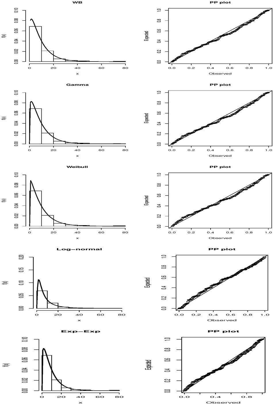
Fitted pdfs and PP plots.
Estimated parameters of the WB, gamma and Weibull distributions.
| Distribution | Parameters | Estimates | Std. Errors | KS | p-value | A | W | AIC | BIC |
|---|---|---|---|---|---|---|---|---|---|
| WB | α | 0.203 | 0.136 | 0.066 | 0.638 | 0.586 | 0.095 | 831.928 | 837.632 |
| θ | 18.938 | 2.701 | |||||||
| Gamma | α | 1.178 | 0.131 | 0.069 | 0.575 | 0.641 | 0.105 | 832.747 | 838.451 |
| θ | 0.125 | 0.017 | |||||||
| Weibull | α | 1.053 | 9.660 | 0.066 | 0.626 | 0.710 | 0.116 | 834.197 | 839.901 |
| θ | 0.068 | 0.857 | |||||||
| Log-normal | μ | 1.764 | 0.095 | 0.065 | 0.643 | 0.870 | 0.131 | 837.295 | 842.999 |
| σ | 1.075 | 0.067 | |||||||
| Exp-Exp | α | 1.223 | 0.149 | 0.068 | 0.586 | 0.597 | 0.097 | 832.181 | 837.885 |
| θ | 0.120 | 0.013 | |||||||
6.2 Application of the WB regression model and its web-tool
Here, we demonstrate the importance of the WB regression model by applying it to the data set on life expectancy of developed and developing countries. The data are taken from the Kaggle platform and are available at https://www.kaggle.com/datasets/kumarajarshi/life-expectancy-who. The variables are measured in the year of 2014 for 131 countries. The research question is Do body mass index (BMI) and country status have an effect on life expectancy? Here, the life expectancy is the dependent variable yi, BMI xi1 and country status (1: developed, 0:developing) xi2 are the independent variables.
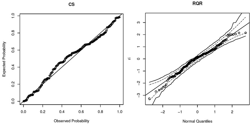
The results of the WB regression model are shown in Table 4. All estimated parameters are found to be statistically significant. Life expectancy in developed countries is exp (0.1274) = 1.1359 times higher than in developing countries. Similarly, for every unit increase in BMI, life expectancy increases by exp (0.0021) = 1.0021 times. Alternatively, if BMI increases by one unit, life expectancy increases by (1.0021–1)×100 = 0.21%. So although BMI is statistically significant, its effect on life expectancy is quite negligible. Table 5 shows the AIC and BIC values for the WB regression model and Figure 3 shows the CS and RQR of the WB regression model. The KS test is also performed on both CS and RQR residuals and the results are reported in Table 6, indicating that both residuals confirm the fit of the WB model to the data.
Estimated parameters of the fitted models.
Results of the WB regression model.
| β0 | β1 | β2 | α | ||||||
|---|---|---|---|---|---|---|---|---|---|
| Estimate | S.E. | p-value | Estimate | S.E. | p-value | Estimate | S.E. | p-value | Estimate |
| 4.1583 | 0.0155 | < 0:001 | 0.0021 | 0.0003 | < 0:001 | 0.1274 | 0.0192 | < 0:001 | 108.1097 |
AIC and BIC values of the WB regression model.
| –ℓ | AIC | BIC |
|---|---|---|
| 605.178 | 1218.356 | 1231.15 |
KS test results for the CS and RQR residuals.
| CS | RQR | ||
|---|---|---|---|
| Test Statistics | p-value | Test Statistics | p-value |
| 0.078 | 0.217 | 0.078 | 0.217 |
Implementing the WB regression model requires advanced knowledge of R or Python. People who want to use this model should maximize the likelihood function using optimization algorithms.
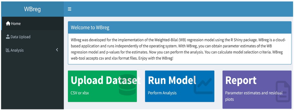
In this study, a cloud-based application called WBreg is developed to enable the widespread use of this model by researchers. WBreg is built using the R Shiny package and available at https://beststat.shinyapps.io/WB2reg that can be easily used. The data set is uploaded to the following website https://github.com/emrahaltun/WBreg. The results can be reproduced by readers and practitioners using the WBreg web application by downloading the data set from the GitHub website.
WBreg application consists of three main panels. These are the home, data upload and analysis panels. The home panel is shown in Figure 4. It gives general information about the programme.
Welcome panel of WBreg.
Figure 5 shows how to load data into the WBreg model. WBreg only accepts two file types. These are the CSV and xlsx file types. After the file has been uploaded, the screen opens where the dependent and independent variables are selected.
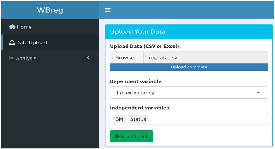
Data upload panel of the WBreg.
The analysis panel consists of three sub-panels. The first panel is given in Figure 6 and contains the parameter estimates of the WBreg model. In this panel, not only the parameter estimates are given, but also the standard errors and p-values.
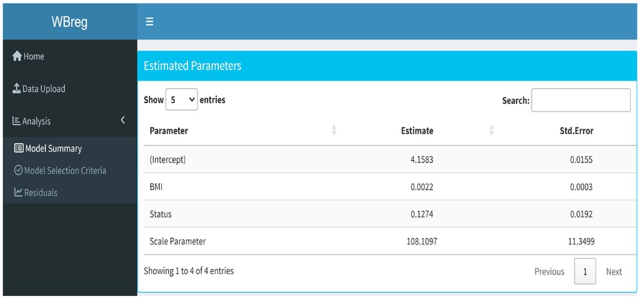
Model summary panel of the WBreg.
In the second sub-panel of the analysis panel, the information criteria are given and shown in Figure 7.
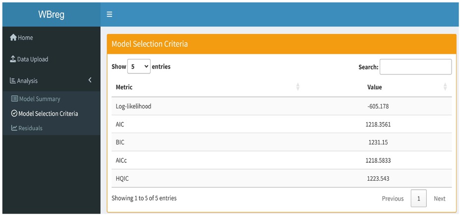
Model selection criteria panel of the WBreg.
Finally, in the third sub-panel of the analysis panel, the results of the residual analysis obtained with CS and RQR are presented. The KS test results for these residuals are also included (see Figure 8).
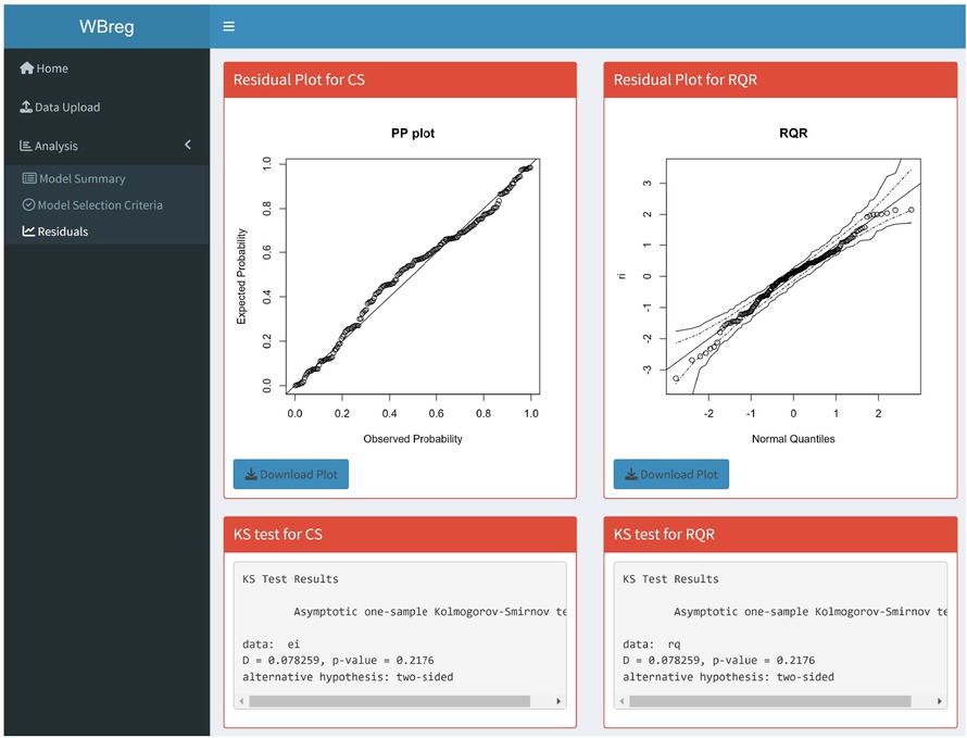
Residual analysis panel of the WBreg.
6.3 Development process of the WBreg
The WBreg user interface is designed using the shinydashboard package to provide a modular, navigable, and user-friendly layout. Several R packages are utilized in the development process.
Data Import and Preprocessing: The readxl [24] package allows users to upload both CSV and Excel files.
Visualization: Base R plotting functions are used for producing PP and QQ plots. The envelopes for QQ plots are constructed using the boot::envelope() [9] function.
The WBreg is deployed on a free public R Shiny Server via shinyapps.io, enabling cloud-based usage without the need for local R/ R Studio installation. The application is developed with reproducibility and simplicity. All calculations are executed within the Shiny server without external dependencies. All outputs such as tables and plots update automatically in response to user inputs.
7 Conclusion
This research introduces a novel weighted distribution called the WB distribution. We have highlighted its important mathematical properties. In addition, its statistical aspect has been extensively studied. Various estimation techniques have been used to determine the unknown parameters of the model. A generalized linear model framework has been constructed under the assumption that the response variable follows the WB distribution. In order to assess the effectiveness of the parameter estimation methods, simulation studies are carried out for both the WB model and the associated regression. In addition, the WBreg tool has been developed and made available to researchers at https://beststat.shinyapps.io/WB2reg. The WBreg tool serves as a powerful tool for implementing the WB regression model.
(Communicated by Gejza Wimmer)
References
[1] Abd-Elrahman, A. M.: Utilizing ordered statistics in lifetime distributions production: a new lifetime distribution and applications, J. Probab. Stat. Sci. 11 (2013), 153–164.Suche in Google Scholar
[2] Abd-Elrahman, A. M.: A new two-parameter lifetime distribution with decreasing, increasing or upside-down bathtub-shaped failure rate, Comm. Statist. Theory Methods 46 (2017), 8865–8880.10.1080/03610926.2016.1193198Suche in Google Scholar
[3] Ahmad, A.—Ahmad, S. P.—Ahmed, A.: Length-biased weighted Lomax distribution: statistical properties and application, Pak. J. Stat. Oper. Res. XII (2016), 245–255.10.18187/pjsor.v12i2.1178Suche in Google Scholar
[4] Aldeni, M.—Lee, C.—Famoye, F.: Families of distributions arising from the quantile of generalized lambda distribution, J. Stat. Distrib. Appl. 4 (2017), 1–18.10.1186/s40488-017-0081-4Suche in Google Scholar
[5] Al-Omari, A. I.—Alsultan, R.—Alomani, G.: Asymmetric right-skewed size-biased Bilal distribution with mathematical properties, reliability analysis, inference and applications, Symmetry 15 (2023), Art. No. 1578.10.3390/sym15081578Suche in Google Scholar
[6] Altun, E.: A new one-parameter discrete distribution with associated regression and integer-valued autoregressive models, Math. Slovaca 70 (2020), 979–994.10.1515/ms-2017-0407Suche in Google Scholar
[7] Altun, E.—El-Morshedy, M.—Eliwa, M. S.: A new regression model for bounded response variable: An alternative to the beta and unit-Lindley regression models, Plos One 16 (2021), 1–15.10.1371/journal.pone.0245627Suche in Google Scholar PubMed PubMed Central
[8] Altun, E.—El-Morshedy, M.—Eliwa, M. S.: A study on discrete Bilal distribution with properties and applications on integer valued autoregressive process, REVSTAT 20 (2022), 501–528.Suche in Google Scholar
[9] Canty, A.—Ripley, B.: boot: Bootstrap R (S-Plus) Functions. R package version 1.3-31, https://CRAN.R-project.org/package=boot 2024.Suche in Google Scholar
[10] Chang, W.—Ribeiro, B. B.: shinydashboard: Create Dashboards with ’Shiny’. R package version 0.7.2, https://CRAN.R-project.org/package=shinydashboard 2021.Suche in Google Scholar
[11] Cox, D. R.—Snell, E. J.: A general definition of residuals, J. R. Stat. Soc. Ser. B. Stat. Methodol. Series B (Methodological) (1968), 248–275.10.1111/j.2517-6161.1968.tb00724.xSuche in Google Scholar
[12] Dey, S.—Dey, T.—Anis, M. Z.: Weighted Weibull distribution: properties and estimation, J. Stat. Theory Pract. 9 (2015), 250–265.10.1080/15598608.2013.875966Suche in Google Scholar
[13] Dunn, P. K.—Smyth, G. K.: Randomized quantile residuals, J. Comput. Graph. Statist. 5 (1996), 236–244.10.1080/10618600.1996.10474708Suche in Google Scholar
[14] Evert, S.—Baroni, M.: zipfR: Word frequency distributions in R. In: Proceedings of the 45th Annual Meeting of the Association for Computational Linguistics, Posters and Demonstrations Sessions, 2007, 29–32, Prague, Czech Republic.10.3115/1557769.1557780Suche in Google Scholar
[15] Ghitany, M. E.—Alqallaf, F.—Al-Mutairi, D. K.—Husain, H. A.: A two-parameter weighted Lindley distribution and its applications to survival data, Math. Comput. Simul. 81 (2011), 1190–1201.10.1016/j.matcom.2010.11.005Suche in Google Scholar
[16] Gupta, R. D.—Kundu, D.: Theory & methods: Generalized exponential distributions, Aust. N. Z. J. Stat. 41 (1999), 173–188.10.1111/1467-842X.00072Suche in Google Scholar
[17] Gupta, R. C.—Kirmani, S. N. U. A..: The role of weighted distributions in stochastic modeling, Comm. Statist. Theory Methods 19 (1990), 3147–3162.10.1080/03610929008830371Suche in Google Scholar
[18] Jain, K.—Singla, N.—Gupta, R.: A weighted version of gamma distribution, Discuss. Math. Probab. Stat. 34 (2014), 89–111.10.7151/dmps.1166Suche in Google Scholar
[19] Lele, S. R.—Keim, J. L.: Weighted distributions and estimation of resource selection probability functions, Ecology 87 (2006), 3021–3028.10.1890/0012-9658(2006)87[3021:WDAEOR]2.0.CO;2Suche in Google Scholar
[20] Patil, G. P.—Rao, C. R.: Weighted distributions and size-biased sampling with applications to wildlife populations and human families, Biometrics (1978), 179–189.10.2307/2530008Suche in Google Scholar
[21] R Core Team: R: A Language and Environment for Statistical Computing, Foundation for Statistical Computing, Vienna, Austria. https://www.R-project.org/.Suche in Google Scholar
[22] Riad, F. H.—Alruwaili, B.—Gemeay, A. M.—Hussam, E.: Statistical modeling for COVID-19 virus spread in Kingdom of Saudi Arabia and Netherlands, Alex. Eng. J. 61 (2022), 9849–9866.10.1016/j.aej.2022.03.015Suche in Google Scholar
[23] Sen, S.—Chandra, N.—Maiti, S. S.: The weighted xgamma distribution: properties and application, J. Reliab. Stat. Stud. 10 (2017), 43–58.Suche in Google Scholar
[24] Wickham, H.—Bryan, J.: readxl: Read Excel Files. R package version 1.4.3, https://CRAN.R-project.org/package=readxl.Suche in Google Scholar
[25] Xie, Y.—Cheng, J.—Tan, X.: DT: A Wrapper of the JavaScript Library ’DataTables’. R package version 0.33; https://CRAN.R-project.org/package=DT.Suche in Google Scholar
Appendix
Proof of Proposition 1. Based on the mixture representation in (2.8), we have
This concludes the proof. □
Proof of Proposition 2. The moment generating function of the WB distribution is defined by M (t) = E (exp (tX)), where X is a random variable with the WB distribution. Based on this classical definition, we have
This end the proof. □
Proof of Proposition 3. Using the following expression: φ (t) = M (it) and Proposition 2, we conclude directly. □
Proof of Proposition 4. The proof can be easily done using the mixture representation of the WB distribution. □
© 2025 Mathematical Institute Slovak Academy of Sciences
This work is licensed under the Creative Commons Attribution 4.0 International License.
Artikel in diesem Heft
- A new categorical equivalence for stone algebras
- On special classes of prime filters in BL-algebras
- A note on characterized and statistically characterized subgroups of 𝕋 = ℝ/ℤ
- New Young-type integral inequalities using composition schemes
- The structure of pseudo-n-uninorms with continuous underlying functions
- Jensen-type inequalities for a second-order differential inequality condition
- A direct proof of the characterization of the convexity of the discrete Choquet integral
- Envelope of plurifinely plurisubharmonic functions and complex Monge-Ampère type equation
- Fekete-Szegö inequalities for Φ-parametric and β-spirllike mappings of complex order in ℂn
- Entire function sharing two values partially with its derivative and a conjecture of Li and Yang
- Oscillatory properties of third-order semi-canonical dynamic equations on time scales via canonical transformation
- Weighted B-summability and positive linear operators
- Some properties and applications of convolution algebras
- On measures of σ-noncompactess in F-spaces
- On the kolmogorov–feller–gut weak law of large numbers for triangular arrays of rowwise and pairwise negatively dependent random variables
- Intermediately trimmed sums of oppenheim expansions: A strong law
- Novel weighted distribution: Properties, applications and web-tool
- On the q-Gamma distribution: Properties and inference
- Finiteorthoatomistic effect algebras and regular algebraic E-test spaces
- Prof. RNDr. Anatolij Dvurečenskij, DrSc. 75th anniversary