Effect of satellite availability and time delay of corrections on position accuracy of differential NavIC
-
Madhu Krishna Karthan
 ,
Devadas Kuna
,
Devadas Kuna

Abstract
The position accuracy of standalone Navigation with Indian Constellation (NavIC) may not be met for certain applications like civil aviation. To improve the position accuracy of the user receiver, the technique used is Differential NavIC, which makes use of Differential corrections. The position accuracy of the user receiver also depends on the satellite availability (i.e. number of satellites available at a certain time instant to estimate the user position) and delay in transmission of differential corrections. In this article, the analysis of differential NavIC using different numbers of visible satellites (satellite availability) and different time delays for transmission of corrections is carried out. For this analysis, three cases are considered, Case I is when all (six) NavIC satellites are visible, Case II is when five satellites (3 Geosynchronous Orbit (GSO) and 2 Geostationary Earth Orbit (GEO)) are visible, and Case III is when five satellites (3 GEO and 2 GSO) are visible. The comparative analysis for these three cases is carried out with respect to the position accuracy parameters and Geometric Dilution of Precision. It is observed that, with the satellite availability in case I and case III, the user receiver accuracy is approximately the same. In case III, the accuracy of the user receiver (3.08 m) is similar to the accuracy (3.09 m) in case I. For time delay in transmission of corrections, different time delays (0, 5, 10, 20, …, 300 s) are considered to observe the effect on the positional accuracy of the user receiver. Due to the increase in this time delay, there is a significant degradation in the user receiver position accuracy of differential NavIC.
1 Introduction
Indian Regional Navigation Satellite System (IRNSS) or NavIC receiver lets a user estimate its position and timing information in and around the Indian region. NavIC signals are affected due to different types of errors in NavIC such as ionosphere, troposphere, receiver clock offset, satellite clock, multipath, and receiver noise (Seeber 2003, Madhu Krishna and Naveen Kumar 2023). Differential NavIC makes use of the corrections to improve the positional accuracy of the users by reducing some of these errors.
1.1 Differential NavIC
A typical Differential NavIC architecture is shown in Figure 1. Differential NavIC consists of a reference station which is located at a known location (which is a well-surveyed location) and a mobile receiver (also called a rover). The reference station estimates the range corrections (difference between pseudo-range and true range) for each NavIC satellite in view, which are transmitted to the rover. The errors that are common to the reference station and the rover can be eliminated as the same set of NavIC satellites are visible to both the receivers. Using these corrections, the rover’s position accuracy is improved (Parkinson 1996, Misra and Enge 2001).

Differential NavIC architecture.
The equation for pseudo-range at the rover receiver (equation (1)) and reference receiver (equation (2)) is
where R
m and R
ref are true ranges (meters) of the rover and reference station, respectively, c is the speed of light in m/s,
The true range R ref is calculated from the known satellite position and predetermined position of the reference station.
where (x sat, y sat, and z sat) is the satellite position (in meters), (x ref , y ref, and z ref) is the fixed position of the reference receiver (in meters).
The differential correction is known by subtracting the true range from the pseudo-range at the reference receiver. The differential correction (ΔD) is
This differential correction is transmitted by the reference station to the rover receiver.
The corrected pseudo-ranges
The above equation is the range correction equation for the rover using which the accuracy of the rover is improved by eliminating the errors which are in common and reducing the other errors (Parkinson 1996).
1.2 Factors affecting satellite availability and its impact on GNSS users
The period of time that a navigation system’s services are available to the user receiver or navigator is referred to as the satellite availability of the navigation system (Seeber 2003, Dutt et al. 2009). Satellites are now an essential component of our contemporary world, facilitating communication, navigation, and data transmission on a global scale. However, a number of factors must be taken into account which can affect the availability of satellite services (Parkinson 1996). Understanding these factors is crucial for the users who rely on satellite technology for their operations.
One key factor affecting satellite availability is orbital congestion. As more satellites are launched into space to meet the growing demand for connectivity, the limited space in certain orbits can become crowded. This congestion can lead to interference and reduced signal quality and has an impact on the availability of satellite services (Misra and Enge 2001, Pan et al. 2019). Atmospheric conditions are another factor. Rain, snow, and storms are examples of weather conditions that can attenuate or scatter satellite signals as they travel through the Earth’s atmosphere. This can result in signal degradation or complete loss of connectivity during severe weather events (Hofmann Wellenhof et al. 1992, Naveen Kumar et al. 2014).
Geographical location also plays a role in satellite availability. Satellites operate within specific coverage areas known as footprints. The size and shape of these footprints vary depending on factors such as satellite altitude and beam characteristics. Therefore, areas located at the edge or outside of a satellite’s footprint may experience weaker signal strength or no coverage at all (Santra et al. 2019, Pan et al. 2022). Technical issues and equipment failures are additional factors that can affect satellite availability. Satellites are complex systems with numerous components that must work together seamlessly to provide reliable services. Any malfunction or failure in these components can disrupt service availability until repairs or replacements are made. Lastly, regulatory restrictions and licensing agreements can impact satellite availability in certain regions or countries (Vasudha and Raju 2017). Governments may impose limitations on frequency bands or require operators to obtain specific licenses before providing services within their jurisdiction.
Therefore, several factors influence the availability of satellite services including orbital congestion, atmospheric conditions, geographical location, technical issues, and regulatory restrictions. Understanding these factors and taking them into account when planning for satellite-based operations or services enable reliable connectivity and minimize disruptions caused by external influences (Sharma et al. 2019).
1.3 Impact of satellite availability on GNSS users
The availability of satellite signals from Global Navigation Satellite Systems (GNSS) like GPS (Global Positioning System), GLONASS (Global Navigation Satellite System), Galileo, and BeiDou and Regional Navigation Satellite Systems (RNSS) like IRNSS and Quasi-Zenith Satellite System, respectively, can significantly impact GNSS and RNSS users in various ways (Rao 2010).
RNSS receivers are intricately linked to satellite availability. The number and positioning of satellites directly impact the precision of location information, with more visible satellites allowing for better triangulation and enhanced accuracy (Nageena Parveen and Siddaiah 2019, Kuter and Kuter 2010). However, in scenarios with limited satellite visibility, such as urban canyons or areas obstructed by tall buildings, signal reliability may diminish due to multipath interference, potentially leading to degraded navigation performance (Specht 2020). The time required for GNSS or RNSS receivers to establish an initial position, known as Time to First Fix (TTFF), can also be prolonged in such conditions (Sundara and Raju 2022). Moreover, the implications extend to safety-critical applications like aviation, where reduced satellite availability may compromise GNSS integrity, risking inaccuracies in navigation information and potentially affecting timing applications crucial for synchronization in various industries (Sivaraj et al. 2017). Therefore, addressing challenges related to satellite visibility is paramount for ensuring the robustness and reliability of GNSS and RNSS systems across diverse applications.
Overall, the impact of satellite availability on GNSS and RNSS users varies depending on the application, location, and the specific GNSS and RNSS constellation being used. GNSS and RNSS users should be aware of potential limitations and consider using alternative positioning technologies or augmentation systems (e.g., Wide Area Augmentation System, European Geostationary Navigation Overlay Service) in areas where satellite availability is limited or compromised.
As per the literature, it is observed that the satellite availability of a standalone navigation system (GNSS or RNSS) has been analysed and no significant work has been carried out on the effect of satellite availability on the position accuracy of differential NavIC. In this article, the effect of satellite availability is analysed for user receiver accuracy of differential NavIC, and the effect of time delay of corrections on position accuracy is analysed for differential NavIC. This work will be helpful to assess the performance of differential NavIC over NavIC service areas.
2 Data acquisition and methodology
The experimental setup to analyse the effect of satellite availability and time delay of corrections on the differential NavIC system is represented in Figure 2. For the analysis, the IGS receiver (A296) is considered as a reference station, and the IGS receiver (A297) is the user receiver. The two receivers’ antennas are separated by a distance of 1.45 m. All the data from the receivers are obtained by considering the receivers to be static. The data obtained from both receivers are of the same date and time (i.e., on 20 September 2019 for 24 h duration, i.e. 86,400 samples). The data used are of RINEX and CSV formats. The reference receiver is set at a well-surveyed location (the coordinates are 17.407°, 78.517°, 450 m, which is obtained by computing the average of the estimated user coordinates in (x, y, z) for the duration of 72 h (Althaf and Hablani 2021, Farrell and Givargis 2000). These coordinates are then converted to latitude, longitude, and height and used as reference station coordinates for the computation of differential corrections.

Experimental setup for Differential NavIC at AGRL Lab.
The steps involved to analyse the effect of satellite availability is depicted in Figure 3 below. The steps involve the calculations at the base station and the user receiver. For satellite availability analysis, three cases are considered. The visibility of all the NavIC satellites ensured is considered as case I and the other two cases as five visible satellites. The availability of satellites along with the orbits is shown in Table 1.

Steps showing calculations at the base station for estimation of differential corrections.
NavIC Satellites with respective PRN and orbit
| Satellite | PRN | Orbit |
|---|---|---|
| IRNSS-1A | I01 | Geosynchronous (IGSO) |
| IRNSS-1B | I02 | Geosynchronous (IGSO) |
| IRNSS-1C | I03 | Geostationary (GEO) |
| IRNSS-1D | I04 | Geosynchronous (IGSO) |
| IRNSS-1E | I05 | Geosynchronous (IGSO) |
| IRNSS-1F | I06 | Geostationary (GEO) |
| IRNSS-1G | I07 | Geostationary (GEO) |
The NavIC satellites with respective Pseudo-Random Noise (PRN) code and the orbit in which the satellite revolves are indicated in Table 1. On the day when the data collected, the satellite IRNSS-1A with PRN I01 orbiting in geosynchronous orbit (GSO) was failed due to atomic clock failure. So, there are six visible satellites on that day.
2.1 At base station
The steps in computing the corrections at the base station (Figure 3) initially involve data extraction. Here, the raw data are converted to RINEX and CSV format from which the required parameters are extracted; then, the satellite positions are estimated and the user position of the base station receiver is computed. For estimation of pseudorange corrections well surveyed location is required which is obtained by taking the average of estimated position of the base station receiver for 72 h. The geometric range is calculated using the satellite position of each NavIC satellite and the surveyed location of the base station. Using the above parameters, the range corrections are estimated for all visible satellites and then transmitted to the user receiver (Madhu Krishna and Naveen Kumar 2023).
2.2 At user receiver
The steps in computing the corrections at the user receiver (Figure 4) initially involve data extraction. The raw data is converted to RINEX and CSV format from which the required parameters for the calculation of satellite position and user position of user receiver are extracted. Here, the differential NavIC analysis is carried out for three cases. Case I: all visible IRNSS satellites (here six visible satellites), Case II: five visible satellites (thee GSO and two GEO), Case III: five visible satellites (three GEO and two GSO). For the above three cases, standalone NavIC 2D accuracy CEP, DRMS, and 2DRMS are computed. Using the range corrections transmitted from the base station receiver, the accuracy is estimated based on the minimum Geometric Dilution of Precision (GDOP) and plotted for all three cases. Further, the position accuracies of standalone NavIC and differential NavIC are compared.

Steps showing calculations at user receiver.
3 Results and discussion
The satellite availability in the context of differential NavIC is analysed by considering three cases. Case I is all visible IRNSS satellites (six visible satellites), Case II is five visible satellites (three GSO and two GEO), and Case III is five visible satellites (three GEO, two GSO).
3.1 Effect of satellite availability on position accuracy of differential NavIC
The effect of satellite availability on position accuracy of differential NavIC is analysed by selecting the different combinations of the satellite by considering minimum GDOP as discussed in the following sections.
3.1.1 Case I: All (six) satellites in view
In the first case, all (six) satellites are visible; the corresponding satellite path and GDOP are shown in Figures 5 and 6, respectively. For all the visible satellites, the satellite positions are plotted in Figure 5. In this figure, the satellite positions of six satellites, of which, three are GEO satellites and three are GSO satellites.

NavIC Satellites path for all (6) visible satellites.

Variation of GDOP for all (six) visible satellites.
Figure 6 shows the GDOP for six visible NavIC satellites in orbit. GDOP is calculated and plotted for 24 h duration, and it is observed that at about 12 and 24 h time, GDOP is higher because of the poor satellite geometry (Rathore 2017). The minimum GDOP value is observed to be 3.72 (at about 5 and 18 h), and the maximum is 4.52 (at about 12 and 24 h). The average value of GDOP is noted to be 3.98.
The position accuracy of standalone NavIC and differential NavIC is plotted in Figure 7(a) and (b), respectively, by considering east error on the x-axis and north error on the y-axis in meters. An East–North-Up (ENU) system is used to represent the NavIC accuracy in terms of east error and north error in meters. The east error and north error are considered to represent the horizontal position error. The data considered are of 24 h duration. Accuracy is plotted with the horizontal accuracy parameters CEP, DRMS, and 2DRMS (Vasudha and Raju 2017).

Position accuracy of user receiver for Case I: (a) standalone NavIC, and (b) differential NavIC.
For standalone NavIC and differential NavIC, the CEP value is observed to be 5.31 and 1.21 m, respectively, which contain the position estimates with a probability of 50%. The DRMS values observed are 7.36 and 1.56 m, which is the radius of the circle with the position estimates with the probability of 65%. The 2DRMS is twice the DRMS value and is observed to be 14.72 and 3.09 m, which is the radius of the circle with the position estimates with a probability of 95% (Madhu Krishna and Naveen Kumar 2023).
3.1.2 Case II: (5 Satellites (three GSO, two GEO))
For case II, the NavIC satellites considered are 3 GSO and 2 GEO satellites. There are three combinations of NavIC satellites are identified which are, combination 1, with PRNs [2 4 5 6 7], combination 2, with PRNs [2 3 4 5 7]. and for combination 3, PRNs are [2 3 4 5 6]. The mean GDOP for these three combinations is 6.76, 7.11, and 4.9, respectively. For these combinations, the satellite path and corresponding GDOP (Figure 8(a) and (b) respectively) are calculated, and the satellite geometry with minimum mean GDOP is considered and used for the analysis. Here, the selected combination of satellites based on minimum GDOP is [2 3 4 5 6].
![Figure 8
(a) NavIC Satellites path for five (three GSO, two GEO) visible satellites (PRN [2 3 4 5 6]), (b) GDOP for five visible satellites (PRN [2 3 4 5 6]).](/document/doi/10.1515/jogs-2022-0169/asset/graphic/j_jogs-2022-0169_fig_008.jpg)
(a) NavIC Satellites path for five (three GSO, two GEO) visible satellites (PRN [2 3 4 5 6]), (b) GDOP for five visible satellites (PRN [2 3 4 5 6]).
The user receiver accuracy of differential NavIC for Case II is plotted in Figure 9(b). The observed accuracy parameters CEP, DRMS, and 2DRMS values are 1.71, 2.19, and 4.38 m, respectively. From the above-observed value, it can be stated that the user position accuracy is improved using the differential positioning technique.

Position accuracy of user receiver for Case II: (a) standalone NavIC, (b) differential NavIC.
3.1.3 Case III: (five Satellites (three GEO, two GSO))
For Case III, the NavIC satellites considered are 3 GEO and 2 GSO satellites. For these satellites, these are three combinations of NavIC satellites are identified which include, for combination 1 the PRNs are [3 4 5 6 7], combination 2, the PRNs are [2 3 5 6 7], and for combination 3, the PRNs are [2 3 4 6 7]. The mean GDOP for these three combinations is 5.41, 4.31, and 4.37, respectively. For these combinations, the satellite path and corresponding GDOP (Figure 10(a) and (b) respectively) are calculated, and the satellite geometry with minimum mean GDOP is considered and used for the analysis. Here, the selected combination of satellites is [2 3 5 6 7].
![Figure 10
(a) NavIC Satellites path for five (three GEO, two GSO) visible satellites (PRN [2 3 5 6 7]), (b) GDOP for five visible satellites (PRN [2 3 5 6 7]).](/document/doi/10.1515/jogs-2022-0169/asset/graphic/j_jogs-2022-0169_fig_010.jpg)
(a) NavIC Satellites path for five (three GEO, two GSO) visible satellites (PRN [2 3 5 6 7]), (b) GDOP for five visible satellites (PRN [2 3 5 6 7]).
The user receiver accuracy of differential NavIC for Case III is plotted in Figure 11(b). The observed accuracy parameters CEP, DRMS, and 2DRMS values are 1.22, 1.54, and 3.08 m, respectively. From the above-observed values, it can be stated that the user position accuracy is improved using the differential positioning technique.
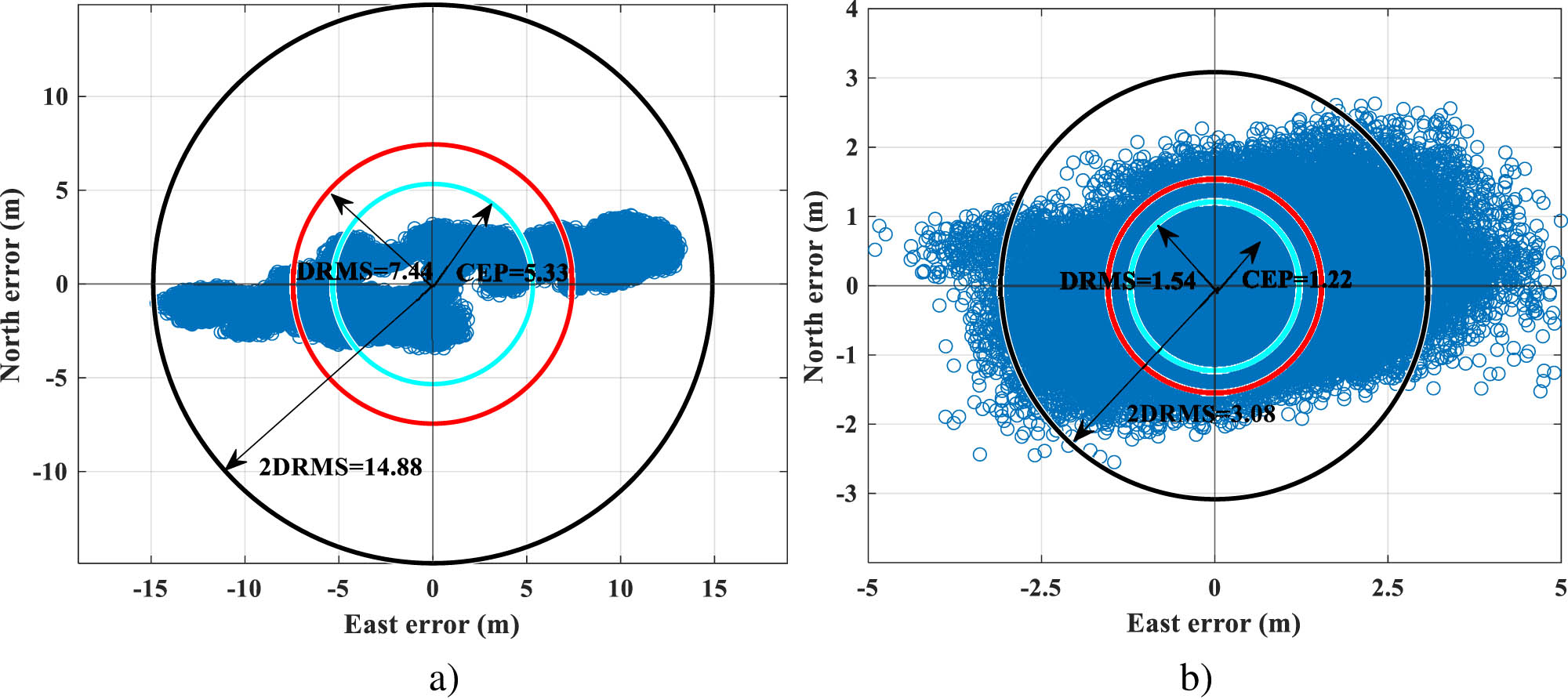
Position accuracy of user receiver for Case III: (a) standalone NavIC, (b) differential NavIC.
The comparison (Table 2) of the accuracy of user receiver for standalone and differential NavIC is represented for Case I, Case II, and Case III. It is observed that, with the satellite availability in Case I (six visible satellites) and Case III (five visible satellites), the rover receiver accuracy is approximately the same. In Case III, even if the available satellites are five, the accuracy of the rover is comparable to the accuracies in Case I.
Comparison of accuracy parameters of rover receiver for standalone and differential NavIC for Case I, Case II, and Case III
| Accuracy Parameters | Case I 6 visible satellites | Case II 3 GSO, 2 GEO | Case III 3 GEO, 2 GSO | |||
|---|---|---|---|---|---|---|
| Standalone (m) | Differential (m) | Standalone (m) | Differential (m) | Standalone (m) | Differential (m) | |
| CEP | 5.31 | 1.21 | 7.05 | 1.71 | 5.33 | 1.22 |
| DRMS | 7.36 | 1.56 | 9.56 | 2.19 | 7.44 | 1.54 |
| 2DRMS | 14.72 | 3.09 | 19.13 | 4.38 | 14.88 | 3.08 |
3.2 Effect of time delay on position accuracy of differential NavIC
To observe the effect of time delay (delay in transmission of range corrections) on the rover position, IRNSS data are collected with the epochs of 1 s. Further, to avoid the effect of residual errors and to focus only on time-delay effects, NavIC data of the same day and time are considered for the base station as well as the rover receiver. The steps involved in the estimation of range corrections and other calculations at the base station and the calculations at user receivers are depicted in Figure 12.

Steps showing calculations at base station and at user receiver.
With respect to different time delay values (0, 5, 10, 20,……300 s), error in rover position is estimated for the epochs under consideration. For differential GPS, the standard delay of 3–4 s is considered (Wang et al. 2016).
For different values of time delay, the position accuracy of the rover is estimated and plotted (Figure 13). It is observed that when the time delay is increased, the accuracy of the rover position is degraded (Table 3).

Time delay vs Accuracy parameters (CEP, DRMS, and 2DRMS).
Minimum, maximum, and standard deviation values of accuracy parameters for different time delay
| Accuracy Parameter | Minimum (m) | Maximum (m) | Standard deviation |
|---|---|---|---|
| CEP | 1.2 | 1.38 | 0.065 |
| DRMS | 1.54 | 1.78 | 0.09 |
| 2DRMS | 3.08 | 3.57 | 0.178 |
4 Conclusions
This article analyses the impact of satellite availability as well as the effect of time delay in transmission of range corrections on the positional accuracy of the NavIC receiver. The effect of satellite availability is analysed by considering three cases, first is by considering all available NavIC satellites, second is by considering five (3 GSO, 2 GEO) visible satellites, and the third is by considering five (three GEO, two GSO) available satellites of different orbits and the comparison is done in terms of accuracy parameters. From these three cases, it is evident that there is an improvement in position accuracy of 78.81, 77.09, and 79.30%, respectively, using differential positioning. For the second and third cases, three different combinations of satellites are considered and GDOP for each is obtained. From the three combinations, the combination of visible satellites which has minimum GDOP is selected and the analysis is carried out. It is observed that, with the satellite availability in Case I (six visible satellites) and Case III (five visible satellites), the user receiver accuracy is approximately the same. In Case III, even though the available satellites are five, the accuracy of the user receiver (3.08 m) is similar to the accuracy (3.09 m) in Case I. The effect of time delay in the transmission of range corrections is analysed by incorporating different delays (0, 5, 10, 20, …., 300 s). It is observed that as the time delay is increased, there is a significant degradation in the user receiver position accuracy of differential NavIC. The research work in this article takes into account the short baseline which aids in the analysis of the user receiver’s position accuracy for medium and long baselines in differential NavIC.
-
Funding information: This research did not receive any specific grant from funding agencies in the public, commercial, or not-for-profit sectors.
-
Author contributions: Madhu Krishna Karthan and Perumalla Naveen Kumar conceived of the presented idea. Madhu Krishna Karthan and Devadas Kuna developed the theory and performed the computations. Perumalla Naveen Kumar encouraged Madhu Krishna Karthan to investigate this specific aspect and supervise the findings of this work. All authors discussed the results and contributed to the final manuscript. The manuscript has been read and approved by the authors.
-
Conflict of interest: The authors declare that they have no known competing financial interests or personal relationships that could have appeared to influence the work reported in this article.
-
Ethics approval: Not applicable.
-
Consent to participate: Not applicable.
-
Consent for publication: Not applicable.
-
Code availability: The source code can be obtained upon reasonable request from the author.
-
Data availability statement: The data sets used and analysed in this study are not publicly available, but the researchers are willing to provide them upon request.
References
Althaf, A. and H. B. Hablani. 2021. “Static baseline estimation using NavIC pseudoranges: A long-term study.” IETE Technical Review 39(4), 827–37. 10.1080/02564602.2021.1912660.Search in Google Scholar
Dutt, V. S. I., G. S. B. Rao, S. S. Rani, S. R. Babu, R. Goswami, and C. U. Kumari. 2009. “Investigation of GDOP for precise user position computation with all satellites in view and optimum four satellite configurations.” Journal of Indian Geophysical Union 13(3), 139–48.Search in Google Scholar
Farrell, J. and T. Givargis. 2000. “Differential GPS reference station algorithm-design and analysis.” IEEE Transactions on Control Systems Technology 8(3), 519–31.10.1109/87.845882Search in Google Scholar
Hofmann Wellenhof, B., H. Lichtenegger, and J. Collins. 1992. GPS theory and practice. New York: Springer-Verlag Wien.Search in Google Scholar
Kuter, N. and S. Kuter. 2010. “Accuracy comparison between GPS and DGPS: A field study at METU campus.” Italian Journal of Remote Sensing 42(3), 3–14.10.5721/ItJRS20104231Search in Google Scholar
Madhu Krishna, K and P. Naveen Kumar. 2023. “Improving the position accuracy of rover receiver using differential positioning in IRNSS.” International Journal of Engineering, Transactions C: Aspects 36(3), 497–504. 10.5829/ije.2023.36.03c.09.Search in Google Scholar
Madhu Krishna, K. and P. Naveen Kumar. 2023. “Comparative analysis of regression algorithms for the prediction of NavIC differential corrections.” Journal of Applied Geodesy 17(4), 415–25. 10.1515/jag-2023-0025.Search in Google Scholar
Misra, P and P. Enge. 2001. Global positioning system. New York: Ganga-Jamuna Press.Search in Google Scholar
Nageena Parveen, S. D. and P. Siddaiah. 2019. “Position error calculations for IRNSS system using pseudo range method.” International Journal of Engineering and Advanced Technology (IJEAT) 8(5), 1085–9.Search in Google Scholar
Naveen Kumar, P., A. D. Sarma, and A. Supraja Reddy. 2014. Modelling of ionospheric time delay of Global Positioning System (GPS) signals using Taylor series expansion for GPS Aided Geo Augmented Navigation applications. IET Radar, Sonar & Navigation 8(9), 1081–90.10.1049/iet-rsn.2013.0351Search in Google Scholar
Pan, L., G. Pei, W. Yu, and Z. Zhang. 2022. “Assessment of IRNSS-only data processing: Availability, Single Frequency SPP and short baseline RTK.” Remote Sensing 14(10), 2462. 10.3390/rs14102462.Search in Google Scholar
Pan, L., X. Zhang, X. Li, X. Li, C. Lu, J. Liu, et al. 2019. “Satellite availability and point positioning accuracy evaluation on a global scale for integration of GPS, GLONASS, BeiDou and Galileo.” Advances in Space Research 63(9), 2696–710.10.1016/j.asr.2017.07.029Search in Google Scholar
Parkinson, B. W. 1996. GPS Theory and Applications, Volume I and Volume II. Washington: American Institute of aeronautics and Astronautics, Inc.Search in Google Scholar
Rao, G. S. 2010. Global navigation satellite system. New Delhi, India: Tata McGraw Hill.Search in Google Scholar
Rathore, C. S. 2017. Planning a GPS Survey Part 2 – Dilution of Precision Errors, February 2017. http://graticules.blogspot.com/2017/02/planning-gps-survey-part-2-dilution-of-html.Search in Google Scholar
Santra, A., S. Mahato, S. Dan, and A. Bose. 2019. “Precision of satellite-based navigation position solution: A review using NavIC data.” Journal of Information and Optimization Sciences 40(8), 1683–91. 10.1080/02522667.2019.1703264.Search in Google Scholar
Seeber, G. 2003. Satellite geodesy. 2nd ed. Berlin, New York: Walter de Gruyter.10.1515/9783110200089Search in Google Scholar
Sharma, A. K., O. B. Gurav, A. Bose, H. P. Gaikwad, G. A. Chavan, A. Santra, et al. 2019. “Potential of IRNSS/NavIC L5 signals for ionospheric studies.” Advances in Space Research 63(10), 3131–8. 10.1016/j.asr.2019.01.029.Search in Google Scholar
Sivaraj, S., U. Swami, R. Babu, and S. C. Rathnakara. 2017. Orbital parameters variations of IRNSS satellites, innovative design and development practices in aerospace and automotive engineering, lecture notes in mechanical engineering. Singapore: Springer. 10.1007/978-981-10-1771-1_57.Search in Google Scholar
Specht, M. 2020. “Statistical distribution analysis of navigation positioning system errors, issue of the empirical sample size.” Sensors 20(24), 7144.10.3390/s20247144Search in Google Scholar PubMed PubMed Central
Sundara, R. and G. Raju. 2022. “Estimation of Indian regional navigation satellite system receiver’s position accuracy in terms of statistical parameters.” SAE Technical Paper 2022-01-6000. 10.4271/2022-01-6000.Search in Google Scholar
Vasudha, M. P. and G. Raju. 2017. “Comparative evaluation of IRNSS performance with special reference to positional accuracy” Gyroscopy Navig 8, 136–49. 10.1134/S2075108717020109.Search in Google Scholar
Wang, L., Z. Li, H. Yuan, J. Zhao, K. Zhou, and C. Yuan. 2016. “Influence of the time-delay of correction for BDS and GPS combined real-time differential positioning.” Electronics Letters 52(12), 1063–5.10.1049/el.2015.4032Search in Google Scholar
© 2024 the author(s), published by De Gruyter
This work is licensed under the Creative Commons Attribution 4.0 International License.
Articles in the same Issue
- Research Articles
- Displacement analysis of the October 30, 2020 (Mw = 6.9), Samos (Aegean Sea) earthquake
- Effect of satellite availability and time delay of corrections on position accuracy of differential NavIC
- Estimating the slip rate in the North Tabriz Fault using focal mechanism data and GPS velocity field
- On initial data in adjustments of the geometric levelling networks (on the mean of paired observations)
- Simulating VLBI observations to BeiDou and Galileo satellites in L-band for frame ties
- GNSS-IR soil moisture estimation using deep learning with Bayesian optimization for hyperparameter tuning
- Characterization of the precision of PPP solutions as a function of latitude and session length
- Possible impact of construction activities around a permanent GNSS station – A time series analysis
- Integrating lidar technology in artisanal and small-scale mining: A comparative study of iPad Pro LiDAR sensor and traditional surveying methods in Ecuador’s artisanal gold mine
- On the topographic bias by harmonic continuation of the geopotential for a spherical sea-level approximation
- Lever arm measurement precision and its impact on exterior orientation parameters in GNSS/IMU integration
- Book Review
- Willi Freeden, M. Zuhair Nashed: Recovery methodologies: Regularization and sampling
- Short Notes
- The exact implementation of a spherical harmonic model for gravimetric quantities
- Special Issue: Nordic Geodetic Commission – NKG 2022 - Part II
- A field test of compact active transponders for InSAR geodesy
- GNSS interference monitoring and detection based on the Swedish CORS network SWEPOS
- Special Issue: 2021 SIRGAS Symposium (Guest Editors: Dr. Maria Virginia Mackern) - Part III
- Geodetic innovation in Chilean mining: The evolution from static to kinematic reference frame in seismic zones