Automatic boomerang attacks search on Rijndael
-
Loïc Rouquette
 ,
Marine Minier
,
Marine Minier

Abstract
Boomerang attacks were introduced in 1999 by Wagner (The boomerang attack. In: Knudsen LR, editor. FSE’99. vol. 1636 of LNCS. Heidelberg: Springer; 1999. p. 156–70) as a powerful tool in differential cryptanalysis of block ciphers, especially dedicated to ciphers with good short differentials. They have been generalized to the related-key case by Biham et al. (Related-key boomerang and rectangle attacks. In: Cramer R, editor. Advances in Cryptology - EUROCRYPT 2005, 24th Annual International Conference on the Theory and Applications of Cryptographic Techniques, Aarhus, Denmark, May 22–26, 2005, Proceedings. vol. 3494 of Lecture Notes in Computer Science. Springer; 2005. p. 507–25. doi: 10.1007/11426639_30). In this article, we show how to adapt the model proposed in 2020 by Delaune et al. (Catching the fastest boomerangs application to SKINNY. IACR Trans Symm Cryptol. 2020;2020(4):104–29) for related-key boomerang attacks on the block cipher SKINNY to the Rijndael case. Rijndael is composed of 25 instances that could be seen as generalizations of the Advanced Encryption Standard. We detail our models and present the results we obtain concerning related-key boomerang attacks on Rijndael. Notably, we present a nine-round attack against Rijndael-128-160, which has 11 rounds and beats all previous cryptanalytic results against Rijdael-128-160.
1 Introduction
The boomerang attack [1] was introduced at FSE’99 as a variant of differential attacks [2]. A cipher
Thus, in Step 1, we compute a truncated related-key boomerang
In this article, we implement and adapt for the Rijndael case [6] the two-step solving process of [5], which was originally proposed for SKINNY to compute related-key boomerang differential characteristics and extended to the advanced encryption standard (AES) in [7]. Note that the models proposed in [7] are quite different as they include a callback search in mixed integer linear programming (MILP) and only concern the AES with probability 1 for the key part. We do not include such a callback search in the present article. Those problems are solved with constraint programming (CP): for the first step, we use Picat-SAT [8], and for the second step, Choco [9][1].
Rijndael is a family of block ciphers (more precisely, it is 25 instances of the same cipher where the block size and the key size vary) originally proposed at the AES competition. But the National Institute of Standards and Technology (NIST) only retained as a standard its 128-bit block version under the key sizes 128, 192, and 256 bits. Studying the security of Rijndael is interesting to enlighten the AES standardization process. The standardization process was completed in 2002. What can be enriched is our understanding of the security of Rijndael and, therefore, of the AES. Among the most interesting results, we obtain a nine-round (over 11 rounds) boomerang related-key differential attack for Rijndael with a block size equal to 128 bits and a key size equal to 160 bits.
When looking at the state of the art concerning the cryptanalysis of Rijndael, some of the results are in the single-key scenario [10–15] or in the related-key scenario [16]. In this article, we obtained a related-key boomerang attack on nine rounds of Rijndael-128-160 working for
The rest of this article is organized as follows: in Section 2, we recall the full description of Rijndael, what is a boomerang attack, and how those attacks are modeled in [5]; in Section 3, we detail the methods and our CP models; in Section 4, we sum up all the related-key boomerang distinguishers we obtained and present two attacks based on the most efficient distinguishers; and finally, in Section 5, we conclude this article.
2 Preliminaries
2.1 Rijndael
Rijndael-
SubBytes is a bytewise transformation that is applied to each byte of the current block using an 8-bit to 8-bit nonlinear S-box, denoted by SBOX. We denote
ShiftRows is a linear mapping that rotates to the left the rows of the current matrix
We denote
MixColumns is a linear multiplication of each column of the current state by a constant matrix
where
AddRoundKey performs a bitwise XOR between the subkey
The number of rounds
|
|
128 | 160 | 192 | 224 | 256 |
|---|---|---|---|---|---|
|
|
10 | 11 | 12 | 13 | 14 |
|
|
11 | 11 | 12 | 13 | 14 |
|
|
12 | 12 | 12 | 13 | 14 |
|
|
13 | 13 | 13 | 13 | 14 |
|
|
14 | 14 | 14 | 14 | 14 |
| Algorithm 1: Rijndael KeySchedule function |
|---|
|
input: A key matrix K of
|
|
output: The expanded key WK of
|
|
for
|
|
|
|
for
|
|
|
| return WK |
The subkeys
Those
2.2 Boomerang attacks
The boomerang attack is a variant of the differential attack that was introduced by David Wagner in 1999 [1].
Given an initial message
In their basic form, boomerang distinguishers are built by rewriting
![Figure 1
A related-key boomerang attack with four keys. This figure is inspired from the one of [20].](/document/doi/10.1515/jmc-2023-0027/asset/graphic/j_jmc-2023-0027_fig_001.jpg)
A related-key boomerang attack with four keys. This figure is inspired from the one of [20].
In [3], the main principle of a boomerang attack has been extended to the related-key case. In addition to the classical boomerang attack, four keys
Recently, Cid et al. [4] have analyzed how to exactly compute the probability in the middle round using a dedicated table called the BCT for SPN ciphers. However, Song et al. [19] and Delaune et al. [5] analyzed more carefully the interactions of the boomerang on several rounds in the middle and introduce some other tables (even in the related-key setting). More precisely, the BCT is only applied on one round (the middle one), whereas the other tables are applied on several rounds (with differences that may not be fixed everywhere). A part of those tables is described in the next subsection for the SPN case.
2.3 Delaune et al.’s model
Delaune et al. [5] proposed a model divided into two steps to search for optimal boomerang distinguishers on SPN ciphers (possibly in the related-key setting). In Step 1, a MILP model searches for truncated boomerangs. Each Step 1 solution is the input of a Step 2 search that tries to instantiate the truncated boomerang with concrete differences to maximize the overall probability of the boomerang distinguisher. Our own search is organized in the same way and divided into the two same steps.
A related-key boomerang attack uses two differential trails; the first one is called the upper trail and determines
For each differential byte
a Boolean variable
a Boolean variable
Constraints are added between
Let us now consider the case of the nonlinear operator Sbox. For each couple of differential bytes (
is added to express the fact that there is an input difference iff there is an output difference, in both upper and lower trails. Then, the following constraints are defined to link together
In addition, if
Each S-box probability is computed with a different table (Differential Distribution Table [DDT], DDT
The goal is to find the values that satisfy all constraints and have the maximal probability. This is done by minimizing the sum of
So, Step 1 outputs boomerang trails considering that the probability computation is the best one even if this best probability cannot be reached when instantiating the exact difference values. This is the role of Step 2 to instantiate the difference values and to compute the best possible probability.
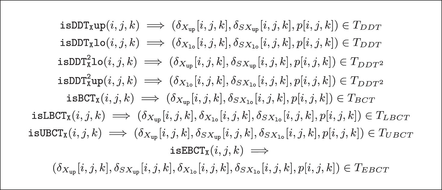
Model 1
Link between binary variables and tables: for each table
3 Automatic search of related-key boomerang distinguishers on Rijndael
In this section, we detail the way we implemented the previous models to fit the case of Rijndael. As in the study by Delaune et al. [5], we divided our search into two steps: in Step 1, we search for truncated boomerang distinguishers with minimal hamming weight, whereas in Step 2, given the output Boolean differences of Step 1, we search for the instantiated boomerang distinguisher with the best probability. We describe in this section each of these two steps.
3.1 Step 1: Automatic search of related-key truncated boomerang distinguishers
As summed up in Section 3, the first step of a related-key boomerang attack may be divided into two parallel searches of related-key truncated differential characteristics (one for the upper trail and the other for the lower trail) and some glue needs to be added for the middle part using the Boolean free variables propagation. For each differential byte
As Rijndael also has Sboxes in the key schedule, we also introduce four Boolean variables for each differential byte
Since Rijndael’s KeySchedule is represented by a two-dimensional matrix, we introduce the same
Constraints are added between
In our model, this constraint becomes:
We do not detail these constraints here and refer the readers to Models 1 and 2 in the study by Rouquette et al. [22].
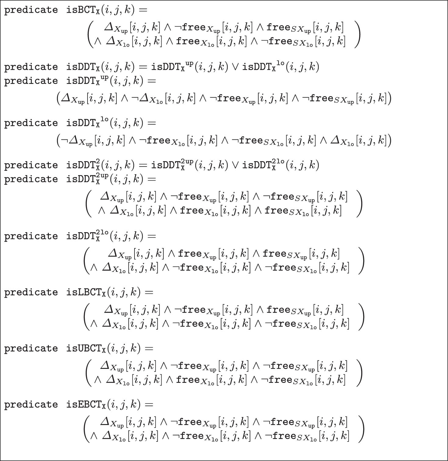
Besides these constraints, we add the new constraints defined in Model 2:
Constraints (B1)–(B5) relate free variables together: (B1) corresponds to AddRoundKey, (B2) corresponds to ShiftRows, (B3) corresponds to MixColumns, and (B4) and (B5) correspond to the KeySchedule. Note that for each round operation (AddRoundKey, ShiftRows, and MixColumns), we have one constraint in the encryption direction for the upper trail, and one constraint in the decryption direction for the lower trail. For the KeySchedule, there are also two constraints, but they are both in the encryption direction because subkeys are all computed from the master key, in both trails.
Constraints (B6) and (B7) define the S-Box rules that glue the two trails as done in the study by Delaune et al. [5].
Constraint (B8) defines the objective function
Implementation. Our Step 1 model has been implemented in MiniZinc [23], which is a high-level and solver-independent language for modeling constraint satisfaction and optimization problems. MiniZinc models are then compiled into FlatZinc, a solver input language that is understood by a wide range of solvers (such as Choco [9], Chuffed [24], or Picat-SAT [8]). In our experiments, we have used Picat-SAT as it is the most efficient for our Step 1 problem. 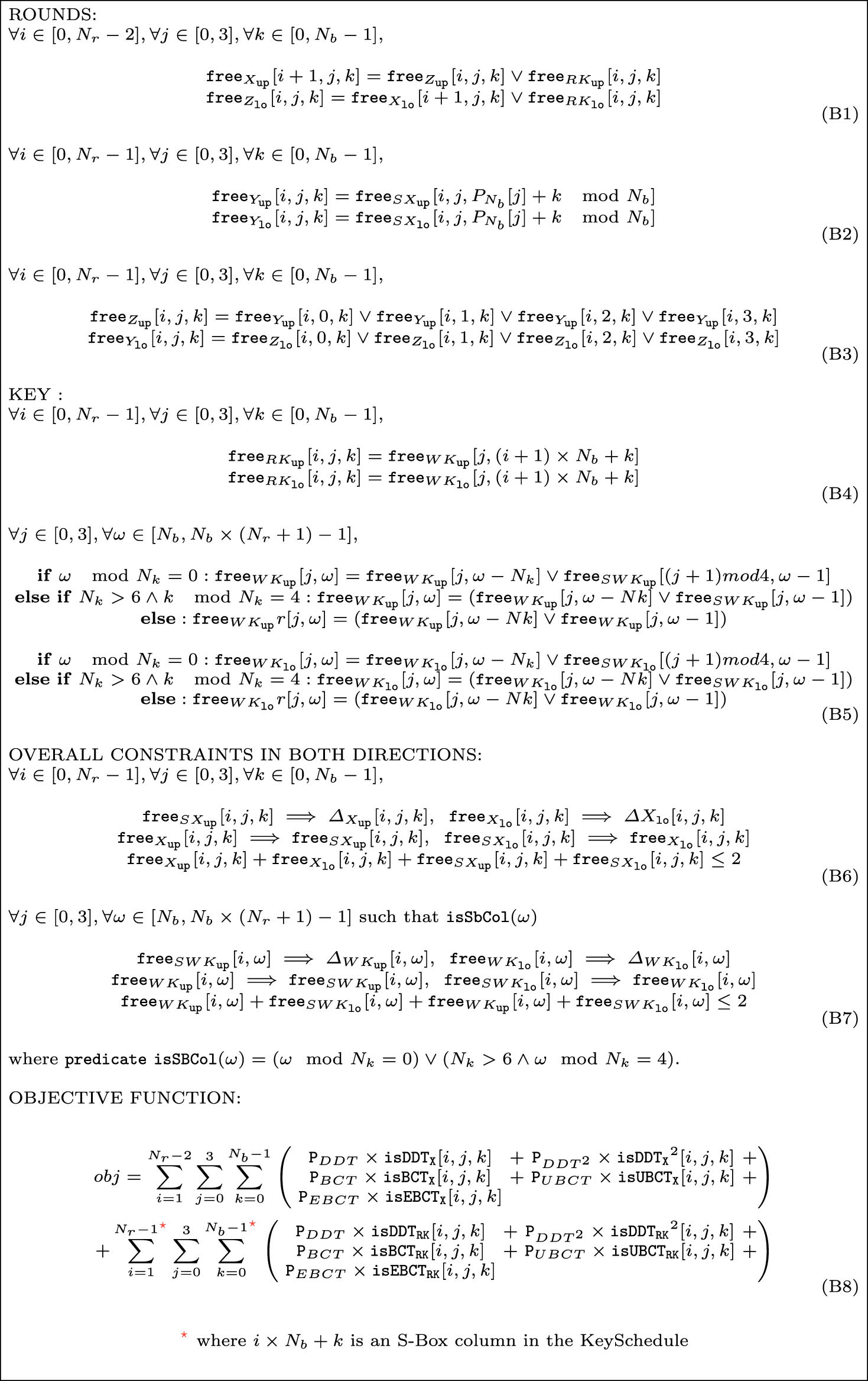
Model 2
Model linking together the free variables for a related-key boomerang computation.
3.2 Step 2: Instantiating the related-key truncated boomerang distinguishers
In this section, we describe how to solve Step 2, which aims at computing the maximal probability of a related-key boomerang distinguisher corresponding to a given truncated distinguisher computed in Step 1 (as explained in the previous section). We first describe the mathematical model and then show how it may be easily implemented using a CP language.
For each round
For S-Box variables, the possible values of this integer variable depend on the value of its associated
Considering that
Finally, we introduce integer variables that represent
Model 3
Constraints that relate
The objective function is then the sum of all
Implementation. Our Step 2 model widely uses table constraints, which are constraints of the form
This model has been implemented with the Choco CP library version 4.10.6 [9].
3.3 Combining the two steps
Step 1 is in fact composed of two different sub-problems: the first one, Step1-Opt, searches for the best possible value of
Note also that Delaune et al. [5], in their original article, also proposed a way to compute the clusters induced. One of the main differences between Rijndael and SKINNY relies on the fact that the linear part of SKINNY is composed of XOR, whereas the one of Rijndael includes multiplication in a finite field. As stated in [25,26], it is out of computational reach to compute such clusters for the AES and thus Rijndael. So, due to the very high computational cost of our method without the cluster computation, we do not include any cluster in our approach.
4 Attacks
4.1 From the distinguisher to the attack
Once an efficient related-key boomerang distinguisher between rounds 1 and
The parameters on which the complexities of an attack are computed are the following ones:
The distinguisher
We add
At the beginning, in the deciphering direction, for
At the end, in the ciphering direction, for
Then, the attack could work on
The attack of [28] works as follows where
Build
For each possible value of the
initialize
partially encrypt each plaintext
insert
use these quartets to determine the correct
The time complexity of the attack is dominated by stage 2.(b) or 2.(d). The complexity, given in the number of encryptions, for stage 2.(b) is
whereas the complexity of stage 2.(d) is
Since stage 2.(b) does partial encryptions over
Then, the success probability
where
To adapt this attack to the case of a nonlinear key-schedule, one has just to compute the correct quartet of keys before the attack. Then, the probability to have a correct quartet only depends on the probability of the S-boxes induced by the KeySchedule and could be directly computed from the distinguisher. The probability of the distinguisher is thus computed without the probability appearing in the KeySchedule. Then, it may be considered as a weak key attack because all the keys could not provide a right quartet. If we denote by
4.2 Results
The Step 1 model is implemented in MiniZinc and run on Picat [8], which uses the Lingeling solver [30]. The Step 2 is implemented in Java, using the Choco library version 4.10.6 [9]. We choose the Picat solver to solve the Step 1 as it is a SAT solver, so is especially suited to problems on Boolean formulae. Previous works like [31] have shown that Picat has good performances on multiple Step 1 models. Since the Step 2 contains a lot of table constraints, it appears that CP solvers are more adapted.
All experiments are run on a virtual machine Ubuntu 18.04.5 LTS x86_64 with an Intel Xeon Gold 5118 processor and 32 Gio of RAM. The requirements are : Java 10.0.12 OpenJDK, Gradle 6.8, MiniZinc 2.5.5, Picat 3.1.2, and Choco 4.10.6. Each instance is run on a single thread.
We put a time out of 6 months. After, those 6 months, the results we obtained are summed up in Table A1 for both Step 1 and Step 2 computations for the related-key boomerang distinguisher on Rijndael.
Even if our models could not reach the largest instances of Rijndael, we obtain the following results:
Rijndael-128-160 with seven rounds, best probability:
Rijndael-160-128 with four rounds, best probability:
Rijndael-192-160 with five rounds, best probability:
Rijndael-160-160 for six rounds with an upper bound equal to
Rijndael-160-192 for seven rounds with an upper bound equal to
Rijndael-160-224 for eight rounds with an upper bound equal to
Rijndael-160-256 for nine rounds with an upper bound equal to
Rijndael-192-128 for four rounds with an upper bound equal to
Rijndael-192-192 for six rounds with an upper bound equal to
Figure 2 displays some statistics about computation times. The upper part of the figure represents which step over the three is the most time consuming, while the lower part of the figure represents the computation time. We can see that the Step 1 (Step1-Opt + Step1-Enum) step is the most time-consuming in general, expected for six (over 37) instances. Moreover, we see that the instances where Step 2 is the most time-consuming are not among the most difficult instances. Hence, improvements should target Step 1 modeling and resolution to improve the overall performances.
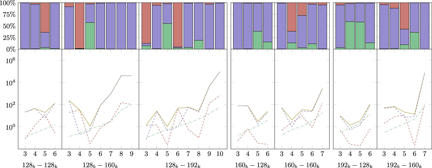
Computation times for instances
 ), Step-1-Enum (
 ), and Step2 (
 ). In the lower part, the chart represents the computation time (in seconds) for each step: Step1-Opt (
 ), Step1-Enum (
 ), and Step2 (
 ) and the cumulative total time (
 ).
).
4.3 Attack on nine rounds of Rijndael-128-160
The nine rounds attack of Rijndael-128-160 is presented in Figure A2 in Appendix B. The distinguisher works for rounds 1 to 8 and has a probability of
Thus, the attack implies the following parameters:
The probability that a right quartet of keys is found is equal to
5 Conclusion
In this article, we have presented the related-key boomerang distinguishers and the related-key boomerang attacks we obtained for some of the 25 instances of the block cipher Rijndael. Among our most significant results, we obtained a nine-round attack on Rijndael-128-160, which has 11 rounds.
However, the computational costs of our models are prohibitive for the largest Rijndael instances. So, we plan to try to improve those models and notably the way the Step 1 is computed to try to reach the missing instances.
Acknowledgements
This work has been partly funded by the French Agence Nationale de la Recherche through the Decrypt project under Contract ANR-18-CE39-0007. Some of the experiments presented in this article were carried out using the LIMOS’ servers. This work has been accepted for presentation at CIFRIS23, the Congress of the Italian association of cryptography “De Componendis Cifris.”
-
Conflict of interest: The authors state that there is no conflict of interest.
-
Code availability: The code produced for the current study is available in the boomerang_rijndael repository: https://gitlab.com/rloic-gitlab/boomerang-rijndael.
Appendix A Overall probabilities
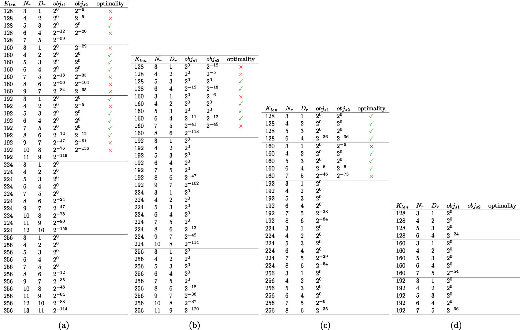
The probabilities found for the different versions of Rijndael. Each table represents a variant Clen of Rijndael. Nr is the number of rounds, Dr is the number of rounds for which we compute the probability of distinction (
B Related-key boomerang distinguisher on nine rounds for Rijndeal-128-160
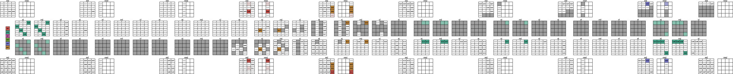
The Rijndael-128-160 nine rounds attack. The distinguisher works for rounds 1–8 and has a probability of
References
[1] Wagner D. The boomerang attack. In: Knudsen LR, editor. FSE’99. vol. 1636 of LNCS. Heidelberg: Springer; 1999. p. 156–70. 10.1007/3-540-48519-8_12Suche in Google Scholar
[2] Biham E, Shamir A. Differential cryptanalysis of DES-like cryptosystems. In: Menezes AJ, Vanstone SA, editors. CRYPTO’90. vol. 537 of LNCS. Heidelberg: Springer; 1991. p. 2–21. 10.1007/3-540-38424-3_1Suche in Google Scholar
[3] Biham E, Dunkelman O, Keller N. Related-key boomerang and rectangle attacks. In: Cramer R, editor. Advances in Cryptology - EUROCRYPT 2005, 24th Annual International Conference on the Theory and Applications of Cryptographic Techniques, Aarhus, Denmark, May 22-26, 2005, Proceedings. vol. 3494 of Lecture Notes in Computer Science. Springer; 2005. p. 507–25. 10.1007/11426639_30. Suche in Google Scholar
[4] Cid C, Huang T, Peyrin T, Sasaki Y, Song L. Boomerang connectivity table: a new cryptanalysis tool. In: Nielsen JB, Rijmen V, editors. EUROCRYPT 2018, Part II. vol. 10821 of LNCS. Heidelberg: Springer; 2018. p. 683–714. 10.1007/978-3-319-78375-8_22Suche in Google Scholar
[5] Delaune S, Derbez P, Vavrille M. Catching the fastest boomerangs application to SKINNY. IACR Trans Symm Cryptol. 2020;2020(4):104–29. 10.46586/tosc.v2020.i4.104-129Suche in Google Scholar
[6] Daemen J, Rijmen V. AES proposal: Rijndael. 1999. Suche in Google Scholar
[7] Derbez P, Euler M, Fouque P, Nguyen PH. Revisiting related-key boomerang attacks on AES using computer-aided tool. In: Agrawal S, Lin D, editors. Advances in Cryptology - ASIACRYPT 2022 - 28th International Conference on the Theory and Application of Cryptology and Information Security, Taipei, Taiwan, December 5-9, 2022, Proceedings, Part III. vol. 13793 of Lecture Notes in Computer Science. Springer; 2022. p. 68–88. 10.1007/978-3-031-22969-5_3. Suche in Google Scholar
[8] Zhou N, Kjellerstrand H. The Picat-SAT compiler. In: Practical Aspects of Declarative Languages - PADL 2016. vol. 9585 of LNCS. Springer; 2016. p. 48–62. 10.1007/978-3-319-28228-2_4Suche in Google Scholar
[9] Prud’homme C, Fages JG, Lorca X. Choco documentation; 2016. http://www.choco-solver.org. Suche in Google Scholar
[10] Jr JN, Pavaaaao IC. Impossible-differential attacks on large-block Rijndael. In: Garay JA, Lenstra AK, Mambo M, Peralta R, editors. Information security, 10th International Conference, ISC 2007. vol. 4779 of LNCS. Springer; 2007. p. 104–17. 10.1007/978-3-540-75496-1_7Suche in Google Scholar
[11] Zhang L, Wu W, Park JH, Koo B, Yeom Y. Improved impossible differential attacks on large-block Rijndael. In: Wu T, Lei C, Rijmen V, Lee D, editors. Information Security, 11th International Conference, ISC 2008. vol. 5222 of LNCS. Springer; 2008. p. 298–315. 10.1007/978-3-540-85886-7_21Suche in Google Scholar
[12] Galice S, Minier M. Improving integral attacks against Rijndael-256 Up to 9 rounds. In: Vaudenay S, editor. Progress in Cryptology - AFRICACRYPT 2008. vol. 5023 of LNCS. Springer; 2008. p. 1–15. 10.1007/978-3-540-68164-9_1Suche in Google Scholar
[13] Wang Q, Gu D, Rijmen V, Liu Y, Chen J, Bogdanov A. Improved impossible differential attacks on large-block Rijndael. In: Kwon T, Lee M, Kwon D, editors. Information security and cryptology - ICISC 2012. vol. 7839 of LNCS. Springer; 2012. p. 126–40. 10.1007/978-3-642-37682-5_10Suche in Google Scholar
[14] Minier M. Improving impossible-differential attacks against Rijndael-160 and Rijndael-224. Des Codes Cryptogr. 2017;82(1–2):117–29. 10.1007/s10623-016-0206-7. Suche in Google Scholar
[15] Liu Y, Shi Y, Gu D, Dai B, Zhao F, Li W, et al. Improved impossible differential cryptanalysis of large-block Rijndael. Sci China Inf Sci. 2019;62(3):32101:1–32101:14. 10.1007/s11432-017-9365-4. Suche in Google Scholar
[16] Wang Q, Liu Z, Toz D, Varici K, Gu D. Related-key rectangle cryptanalysis of Rijndael-160 and Rijndael-192. IET Inf Secur. 2015;9(5):266–76. 10.1049/iet-ifs.2014.0380. Suche in Google Scholar
[17] Daemen J, Rijmen V. The design of Rijndael: AES – the Advanced Encryption Standard. Berlin; London: Springer; 2002. OCLC: 751525895. 10.1007/978-3-662-04722-4_1Suche in Google Scholar
[18] Advanced Encryption Standard (AES); 2001. National Institute of Standards and Technology (NIST), FIPS PUB 197, U.S. Department of Commerce. Suche in Google Scholar
[19] Song L, Qin X, Hu L. Boomerang connectivity table revisited. Application to SKINNY and AES. IACR Trans Symmetric Cryptol. 2019;2019(1):118–41. 10.13154/tosc.v2019.i1.118-141. Suche in Google Scholar
[20] Jean J. TikZ for Cryptographers; 2016. https://www.iacr.org/authors/tikz/. Suche in Google Scholar
[21] Gerault D, Lafourcade P, Minier M, Solnon C. Computing AES related-key differential characteristics with constraint programming. Artif Intell. 2020 Jan;278:103183. https://linkinghub.elsevier.com/retrieve/pii/S0004370218303631. 10.1016/j.artint.2019.103183Suche in Google Scholar
[22] Rouquette L, Gérault D, Minier M, Solnon C. And Rijndael: automatic related-key differential analysis of Rijndael. In: Batina L, Daemen J, editors. Progress in Cryptology - AFRICACRYPT 2022: 13th International Conference on Cryptology in Africa, AFRICACRYPT 2022, Fes, Morocco, July 18–20, 2022, Proceedings. vol. 13503 of LNCS. Springer Nature Switzerland; 2022. p. 150–75. 10.1007/978-3-031-17433-9_7Suche in Google Scholar
[23] Nethercote N, Stuckey PJ, Becket R, Brand S, Duck GJ, Tack G. MiniZinc: towards a standard CP modelling language. In: Principles and Practice of Constraint Programming - CP 2007. vol. 4741 of LNCS. Springer; 2007. p. 529–43. 10.1007/978-3-540-74970-7_38Suche in Google Scholar
[24] Chu G, Stuckey PJ. Chuffed solver description; 2014. http://www.minizinc.org/challenge2014/description_chuffed.txt. Suche in Google Scholar
[25] Canteaut A, Roué J. On the behaviors of affine equivalent Sboxes regarding differential and linear attacks. In: Oswald E, Fischlin M, editors. Advances in Cryptology - EUROCRYPT 2015 - 34th Annual International Conference on the Theory and Applications of Cryptographic Techniques, Sofia, Bulgaria, April 26-30, 2015, Proceedings, Part I. vol. 9056 of Lecture Notes in Computer Science. Springer; 2015. p. 45–74. 10.1007/978-3-662-46800-5_3. Suche in Google Scholar
[26] Daemen J, Rijmen V. Understanding two-round differentials in AES. In: Prisco RD, Yung M, editors. Security and Cryptography for Networks, 5th International Conference, SCN 2006, Maiori, Italy, September 6–8, 2006, Proceedings. vol. 4116 of Lecture Notes in Computer Science. Springer; 2006. p. 78–94. 10.1007/11832072_6. Suche in Google Scholar
[27] Dong X, Qin L, Sun S, Wang X. Key guessing strategies for linear key-schedule algorithms in rectangle attacks. IACR Cryptol ePrint Arch. 2021;2021:856. https://eprint.iacr.org/2021/856. Suche in Google Scholar
[28] Zhao B, Dong X, Meier W, Jia K, Wang G. Generalized related-key rectangle attacks on block ciphers with linear key schedule: applications to SKINNY and GIFT. Des Codes Cryptogr. 2020;88(6):1103–26. 10.1007/s10623-020-00730-1. Suche in Google Scholar
[29] Selçuk AA. On probability of success in linear and differential cryptanalysis. J Cryptol. 2008 Jan;21(1):131–47. 10.1007/s00145-007-9013-7Suche in Google Scholar
[30] Biere A. Lingeling and friends at the SAT Competition 2011. 2011. Institut for Formal Models and Verification, Johannes Kepler University. https://epub.jku.at/obvulioa/content/titleinfo/5973538. Suche in Google Scholar
[31] Libralesso L, Delobel F, Lafourcade P, Solnon C. Automatic generation of declarative models for differential cryptanalysis. In: Michel LD, editor. 27th International Conference on Principles and Practice of Constraint Programming, CP 2021, Montpellier, France (Virtual Conference), October 25–29, 2021. vol. 210 of LIPIcs. Schloss Dagstuhl - Leibniz-Zentrum für Informatik; 2021. p. 40:1–40:18. https://doi.org/10.4230/LIPIcs.CP.2021.40. Suche in Google Scholar
[32] Biryukov A, Nikolic I. Automatic search for related-key differential characteristics in byte-oriented block Ciphers: application to AES, Camellia, Khazad and others. In: Advances in Cryptology - EUROCRYPT 2010. vol. 6110 of LNCS. Springer; 2010. p. 322–44. 10.1007/978-3-642-13190-5_17Suche in Google Scholar
© 2024 the author(s), published by De Gruyter
This work is licensed under the Creative Commons Attribution 4.0 International License.
Artikel in diesem Heft
- Regular Article
- The dihedral hidden subgroup problem
- Characterizing the upper bound on the transparency order of (n, m)-functions
- Tropical cryptography III: Digital signatures
- A security analysis of two classes of RSA-like cryptosystems
- On the quantum security of high-dimensional RSA protocol
- On implementation of Stickel's key exchange protocol over max-min and max-T semirings
- Revocable policy-based chameleon hash using lattices
- Revisiting linearly extended discrete functions
- Special Issue based on CIFRIS23
- Special issue based on the CIFRIS 2023 conference
- On linear codes with random multiplier vectors and the maximum trace dimension property
- Group structure of elliptic curves over ℤ/Nℤ
- mRLWE-CP-ABE: A revocable CP-ABE for post-quantum cryptography
- On the Black-Box impossibility of multi-designated verifiers signature schemes from ring signature schemes
- Searchable encryption with randomized ciphertext and randomized keyword search
- Differential experiments using parallel alternative operations
- On a generalization of the Deligne–Lusztig curve of Suzuki type and application to AG codes
- Automatic boomerang attacks search on Rijndael
- Efficiency of SIDH-based signatures (yes, SIDH)
- Cryptanalysis of a privacy-preserving authentication scheme based on private set intersection