Decision-theoretic foundations for statistical causality: Response to Shpitser

Philip Dawid

doi:10.1515/jci-2022-0013

Artikel Open Access

Decision-theoretic foundations for statistical causality: Response to Shpitser

Philip Dawid

Veröffentlicht/Copyright: 16. August 2022

Veröffentlicht von

Veröffentlichen auch Sie bei De Gruyter Brill

Manuskript einreichen Informationen für Autor*innen

Aus der Zeitschrift Journal of Causal Inference Band 10 Heft 1

Abstract

I thank Ilya Shpitser for his comments on my article, and discuss the use of models with restricted interventions.

Keywords: causal inference; extended conditional independence; front-door formula; graphical models; intention to treat; partially intervenable model

MSC 2010: 62A01; 62C99

1 Introduction

It has been a pleasure to read Ilya Shpitser’s thoughtful discussion [1] of my article [2]. I am delighted to see how readily he has taken the DT approach to statistical causality, and he has demonstrated admirable facility in manipulating it. As he notes, I have been advocating and exploring this approach for over 20 years, though with disappointingly little causal effect. I hope that excellent contributions such as his to this area will help to spread the good word more widely.

He says: “It is thus not clear what role an explicitly decision-focused type of causal inference would play in the ecosystem in which empirical science is done today.” This is a fair point, but one that can just as easily be directed at the other current formal frameworks, such as potential outcomes and graphical models. In my partial defence, I could point to the importance, in this ecosystem, of the ability to transport [3] causal findings from one context (e.g. that of an experimental or observational study) to another (e.g. “real-world” behaviour in a population of interest). This typically involves making an invariance assumption [4] that certain marginal or conditional distributions are the same in all relevant contexts. DT focuses on just this kind of assumption, where a conditional distribution, e.g. of Y given X , is taken to be the same, across observational and interventional regimes – a property that can be helpfully described by means of extended conditional independence (ECI), notated as Y ⊥ ⊥ F ∣ X , where F indicates the regime. More general problems of transportability, e.g. to the “real-world,” can be described and handled with exactly the same machinery – the only, very minor, difference being a widening of the interpretative scope of a non-stochastic “decision variable” such as F to encompass more general kinds of context [5, Section 11.4.1].

2 Graphs or algebra?

Shpitser asks: “Why is the DT approach based on directed acyclic graphs?” To which I answer: “It isn’t.” It is based, as indicated above, on the identification of transportable distributional components, which are then described in terms of ECI, and manipulated using the algebra of conditional independence. Given an initial set of assumptions, expressed as ECI properties, we can uncover their implications by repeated application of the ECI axioms (properties P1–P5 in my article). Sometimes our assumptions can be represented and manipulated (using d -separation) by an augmented directed acyclic graph (DAG); sometimes by a more general kind of graph (e.g. a chain graph: see Example 11.2 of [6]); and sometimes there is no graphical representation whatsoever. But the DT approach never requires that our conditional independence properties be representable in graphical form – and even when they are, everything that can be deduced can be deduced using algebra alone. There may even be advantages to confining attention to the algebra, given the ease with which graphs can be misleading and are regularly misunderstood [6].

That said, DAG representations of causal problems are ubiquitous, and, when available, are much easier to understand and apply than the stark algebra. I have used and investigated DAGs in my article for these reasons – but they are never necessary.

3 Identification theory

Most of Shpitser’s discussion concerns an incidental aspect of DT: formal intervention variables are introduced only when they represent genuine real-world interventions. To me this seems only natural, though I am perhaps not quite as committed to it as he appears to be: I would not be averse to making purely instrumental use of an artificial intervention variable, if that could be shown to facilitate analysis. Nevertheless, I always favour a minimalist approach, so was happy to learn from him that, when applying (the DT version of) do-calculus, it is never necessary to incorporate intervention variables other than those required to give meaning to the query at hand. Shpitser’s illustrations of this, for the front-door and napkin problems, are very pleasing.

Some time ago, Vanessa Didelez and I developed an argument for the front-door criterion (see [7], Section 5.4.2), as modelled by Figure 1. Like Figure 1(a) of [1], this involves intervention only on A . But it differs from that representation in two ways. The first is the removal of the covariate C : this is entirely inconsequential, since the whole argument could be carried out conditional on covariates. The second is that (similar to the move from Figure 9 to Figure 10 in [2]) we have ignored the intention-to-treat (ITT) variable A ∗ , so representing only the ECIs between the domain variables H , A , M , and Y , viz.

(1) H ⊥ ⊥ F A .

(2) M ⊥ ⊥ ( H , F A ) ∣ A .

(3) Y ⊥ ⊥ ( A , F A ) ∣ ( H , M ) .

In addition, we have the deterministic relation

(4) F A = a ⇒ A = a .

All further analysis is by purely algebraic application of properties (1)–(4).

For simplicity, we suppose all variables are discrete. We write p ∅ ( ⋅ ) for p ( ⋅ ; F A = ∅ ) , and p a ( ⋅ ) for p ( ⋅ ; F A = a ) . Note that, by (4),

(5) p a ( ⋅ ) = p a ( ⋅ ∣ A = a ) .

Figure 1

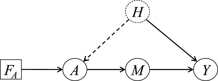
Augmented DAG for the front-door criterion.

Lemma 1

Consider the following function q ( y ∣ m ) of the joint distribution under F A = ∅ :

q ( y ∣ m ) = ∑ h ∑ a p ∅ ( y ∣ h , m ) p ∅ ( a , h ) .

Then

(6) q ( y ∣ m ) = ∑ h p ∅ ( y ∣ h , m ) p ∅ ( h )

(7) = ∑ a p ∅ ( y ∣ a , m ) p ∅ ( a ) .

Proof

We trivially have q ( y ∣ m ) = ∑ h p ∅ ( y ∣ h , m ) ∑ a p ∅ ( a , h ) , yielding (6).

Also,

(8) q ( y ∣ m ) = ∑ h ∑ a p ∅ ( y ∣ a , h , m ) p ∅ ( a ) p ∅ ( h ∣ a )

(9) = ∑ a p ∅ ( a ) ∑ h p ∅ ( y ∣ a , h , m ) p ∅ ( h ∣ a , m ) = ∑ a p ∅ ( y ∣ a , m ) p ∅ ( a ) ,

where (8) holds because, by (3), Y ⊥ ⊥ M ∣ ( A , H , F A = ∅ ) ; while (9) holds because, by (2), H ⊥ ⊥ M ∣ ( A , F A = ∅ ) .□

If we could intervene on M , then (by application of the back-door formula, first accounting for H , and then for A ), each of (6) and (7) would give the causal effect of M on Y ; but we do not need to invoke artificial interventions to show that the two purely observational expressions (6) and (7) are equal.

Theorem 1

(10) p a ( y ) = ∑ m p ∅ ( m ∣ a ) ∑ a ′ p ∅ ( y ∣ a ′ , m ) p ∅ ( a ′ ) .

This is the front-door formula, yielding an expression for p a ( y ) that depends entirely on the observational distribution of the observable variables ( A , Y , M ) .

Proof

From (5) and (2), p a ( m ∣ h ) = p a ( m ∣ h , a ) = p a ( m ∣ a ) . Thus,

p a ( y ) = ∑ m ∑ h p a ( y ∣ h , m ) p a ( m ∣ a ) p a ( h ) , = ∑ m p ∅ ( m ∣ a ) ∑ h p ∅ ( y ∣ h , m ) p ∅ ( h )

since p a ( h ) = p ∅ ( h ) by (1); p a ( m ∣ a ) = p ∅ ( m ∣ a ) since M ⊥ ⊥ F A ∣ A , by (2); and p a ( y ∣ h , m ) = p ∅ ( y ∣ h , m ) , since Y ⊥ ⊥ F A ∣ ( H , M ) , by (3).

Finally, by Lemma 1 the second sum can be replaced by ∑ a ′ p ∅ ( y ∣ a ′ , m ) p ∅ ( a ′ ) .□

The above argument differs from that of Shpitser’s DT argument: it uses H but ignores A ∗ , while his uses A ∗ and ignores H . Which of these is to be preferred is a matter of taste. I like his version, and so had hoped it might turn out that, in the general case, by explicit introduction of ITT variables we could avoid explicit consideration of unobserved domain variables; but Shpitser’s analysis of the napkin problem appears to require both kinds of variable. I conjecture, however, that, for a general identification argument, where we only model interventions of genuine interest, it will be possible to confine attention to the ECI relationships between domain variables, both observed and unobserved (as well as definitional relationships such as (5)), and avoid consideration of ITT variables.

Conflict of interest: Prof. Philip Dawid is a member of the Editorial Board in the Journal of Causal Inference but was not involved in the review process of this article.

References

[1] Shpitser I. Comment on: “Decision-theoretic foundations for statistical causality”. J Causal Inference 2022;10:190–6. 10.1515/jci-2021-0056Suche in Google Scholar

[2] Dawid AP. Decision-theoretic foundations for statistical causality. J Causal Inference. 2021;9:39–77. 10.1515/jci-2020-0008. Suche in Google Scholar

[3] Pearl J, Bareinboim E. Transportability of causal and statistical relations: a formal approach. In: Burgard W, Roth D, editors, Proceedings of the 25th AAAI Conference on Artificial Intelligence. Menlo Park, CA: AAAI Press; 2011. p. 247–54. http://www.aaai.org/ocs/index.php/AAAI/AAAI11/paper/view/3769/386410.1109/ICDMW.2011.169Suche in Google Scholar

[4] Bühlmann P. Invariance, causality and robustness (with Discussion). Statistical Sci. 2020;35:404–36. 10.1214/19-STS721Suche in Google Scholar

[5] Dawid AP. Counterfactuals, hypotheticals and potential responses: a philosophical examination of statistical causality. In: Russo F, Williamson J, editors. Causality and Probability in the Sciences. Volume 5 of Texts in Philosophy. London: College Publications. 2007. p. 503–32. Suche in Google Scholar

[6] Dawid AP. Beware of the DAG!. In: Guyon I, Janzing D, Schölkopf B, editors. Proceedings of the NIPS 2008 Workshop on Causality. Volume 6 of Journal of Machine Learning Research Workshop and Conference Proceedings. Brookline, MA: Microtome Publishing; 2010. p. 59–86. http://tinyurl.com/33va7tm. Suche in Google Scholar

[7] Didelez V. Causal concepts and graphical models. In: Maathuis M, Drton M, Lauritzen S, Wainwright M. editors. Handbook of Graphical Models. Chapter 15. 1st edition. Boca Raton, FL; CRC Press; 2018. p. 353–80. 10.1201/9780429463976-15Suche in Google Scholar

Received: 2022-02-18

Accepted: 2022-07-22

Published Online: 2022-08-16

This work is licensed under the Creative Commons Attribution 4.0 International License.

Artikel in diesem Heft

https://doi.org/10.1515/jci-2022-0013

Schlagwörter für diesen Artikel

causal inference; extended conditional independence; front-door formula; graphical models; intention to treat; partially intervenable model

Creative Commons

BY 4.0