Comment on: “Decision-theoretic foundations for statistical causality”

1 Causal inference versus assisted decision-making

Equating causal inference in the DT framework with assisted decision making seems to be mismatched with the rationale for much applied causal inference work. Indeed, causal inference methods allow the use of observational data to mimic an RCT. Many randomized and observational studies are performed primarily to establish a scientifically interesting relationship between variables, rather than to assist with a particular decision. In practice, such studies provide support for actual decisions either not at all, or only indirectly, and perhaps only in the context of a large collection of similar studies which together form sufficiently strong evidence to merit change in government policy, or modification of clinical practice.

That this is the role causal inference plays in practice is explicitly acknowledged by many empirical disciplines, which establish hierarchies of evidence, with meta analyses of randomized trials forming the most convincing type of evidence for a causal claim. It is thus not clear what role an explicitly decision-focused type of causal inference would play in the ecosystem in which empirical science is done today.

2 Why is the DT approach based on directed acyclic graphs (DAGs)?

Like other frameworks for causal inference, specifically Pearl’s approach [7], and the approach based on SWIGs [6], the DT framework is based on DAGs. In the case of Pearl’s approach, the use of DAGs follows naturally from non-parametric structural equation semantics, where the output variable of each structural equation may be viewed as a child of all input variables in the graph.

Similarly, an SWIG causal model in which all variables can be intervened on assumes (1) a total ordering among variables, and (2) a set of one-step-ahead counterfactuals, from which all other counterfactuals making up the causal model are defined. These assumptions immediately lead to a DAG representation of a causal model in ref. [5] called the finest causally interpretable structured tree graph (FCISTG) as detailed as the data (that assumes all variables can be intervened on) [9]. Note that general structured tree graph models are defined given a subset of variables in the problem on which interventions may be conceptualized. Given such a subset, an FCISTG model is only considered finest and as detailed as the data if restrictions defining it involve interventions on all variables that permit interventions, and not otherwise [5].

Unlike these formalisms, however, the only part of the DT approach that seems to entail a DAG structure is the relationship between the regime indicator F A , the intention to treat variable A ∗ , and the treatment variable A . Specifically, the way these variables are defined implies they can be visualized as a DAG collider structure: F A → A ← A ∗ . However, as far as I can see, nothing in the framework requires that the way these variables relate to other variables in the system should be represented by a DAG, or indeed by any kind of graphical model at all!^[1]

While DAGs allow an analytically convenient Markov property via the d-separation criterion, analytical convenience does not seem to me to be a good standard for choosing a representation of a causal model. However, if it is true that the DT framework may be formulated for other types of graphical models (or even without graphs), this may be a strength rather than a weakness of the formalism. Indeed, more general types of graphs have been used to represent various complications that DAGs are ill suited for capturing [10,11, 12,13]. Incorporating these graphs into existing causal frameworks is often challenging. For example, defining a causal chain graph model^[2] entailed a generalization of structural equation replacement semantics for DAGs to models allowing samplers that reach equilibrium [10]. In contrast, such extensions may be much easier in the DT framework, as it seems to be largely graph structure agnostic. Indeed, Professor Dawid discussed extensions of the DT framework to chain graphs in one particular special case in ref. [14].

3 General identification theory

The DT framework has, like the CISTG approach in ref. [5], the (in my opinion desirable) property of being only partially causal. To illustrate why this property can create difficulties for the fundamental problem of causal effect identification, I will consider identification of an interventional distribution in the DT framework version of the front-door model [7,15], as shown in Figure 1(a). Unlike the derivation in ref. [16], the derivation below makes no mention of the hidden variable H in the problem, or restrictions involving this variable.

Figure 1

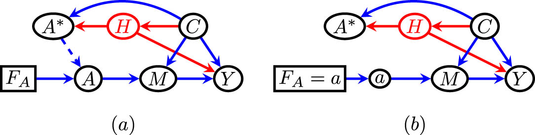
(a) The front-door model graph represented in the decision-theoretic framework. The dashed edge represents a context-specific relation between the intention to treat version of the treatment ( A ∗ ) and the treatment itself ( A ). This relationship disappears if F A ≠ ∅ . (b) The edge subgraph of (a) showing context-specific independences that occur when F A ≠ ∅ .

A number of interesting observations follow from this derivation.

1. While the intention to treat variable A ∗ is not necessarily observable in interventional regimes (where F A = a ), a distribution which involves both F A being set to a and A ∗ arises in this derivation, on line 5. This does not create a problem provided that the derivation ends with a functional that is fully observed, as in ref. [5]. This is in contrast to identification derivations in some frameworks, which are generally formulated in such a way that every intermediate step involves distributions that are fully observed (if perhaps in some interventional context).

2. A context-specific independence is used on line 6. Specifically, it is only the case that the intention to treat variable A ∗ is independent of the mediator M given C in the interventional regime, not the idle regime. This is because A ∗ and M are connected by a d -connected path that disappears only under the interventional regime. This is easy to see by examining Figure 1(b), which represents d -separation relationships in any interventional context F A = a .

3. Note also that a seemingly reasonable replacement of the term p ( a ∗ ∣ m , c , F A = a ) on line 5 by the term p ( a ∗ ∣ m , c , F A = ∅ ) is not valid, even though there are no d -connecting paths connecting A ∗ and F A in Figure 1(b). This is because d-separation of these vertices relies on F A being equal to a . Under the idle regime, F A and A ∗ are d-connected given C and M , due to the collider A ∗ → A ← F A with a conditioned descendant ( M ). In other words, this is yet another consequence of context-specific independence assumptions in the DT framework.

4. Another curious manifestation of this phenomenon is that under the given model Y ⊥ ⊥ F A ∣ M , C , F A ≠ ∅ , even if A has a continuous state space. Note that this independence explicitly excludes cases where F A = ∅ . In other words, the conditional distribution p ( Y ∣ M , C , F A = a ) is not sensitive to values attained by F A – provided these values correspond to the interventional regime.

5. The functional on the last line contains only observed quantities, and therefore serves as the identifying functional for p ( Y ∣ F A = a ) . Indeed, it is easy to verify that this functional is a decision-theoretic framework analogue of the front-door functional [15].

6. Professor Dawid points out that intention to treat variables behave as covariates. In the identifying functional A ∗ indeed behaves as a covariate. In fact, the first term in the identifying functional on the last line resembles the adjustment functional where A ∗ serves as covariates being adjusted for, and M serves the role of the treatment variable.

7. Despite the previous point, and in keeping with the DT framework being partly causal, the above derivation did not assume the mediator M may be intervened on, unlike typical derivations of the front-door functionals using the d o ( ) -operator or potential outcome notation, such as the one below, using potential outcomes:

   p ( Y ( a ) ) = ∑ c , m p ( Y ( a ) ∣ M ( a ) = m , c ) p ( M ( a ) = m ∣ c ) p ( c ) = ∑ c , m p ( Y ( a ) ∣ M ( a ) = m , c ) p ( M ( a ) = m ∣ a , c ) p ( c ) = ∑ c , m p ( Y ( a ) ∣ M ( a ) = m , c ) p ( m ∣ a , c ) p ( c ) = ∑ c , m ∑ a ∗ p ( Y ( a ) ∣ M ( a ) = m , c , a ∗ ) p ( a ∗ ∣ M ( a ) = m , c ) p ( m ∣ a , c ) p ( c ) = ∑ c , m ∑ a ∗ p ( Y ( a ) ∣ M ( a ) = m , c , a ∗ ) p ( a ∗ ∣ c ) p ( m ∣ a , c ) p ( c ) = ∑ c , m ∑ a ∗ p ( Y ( a , m ) ∣ c , a ∗ ) p ( a ∗ ∣ c ) p ( m ∣ a , c ) p ( c ) = ∑ c , m ∑ a ∗ p ( Y ( m ) ∣ c , a ∗ ) p ( a ∗ ∣ c ) p ( m ∣ a , c ) p ( c ) = ∑ c , m ∑ a ∗ p ( Y ( m ) ∣ m , c , a ∗ ) p ( a ∗ ∣ c ) p ( m ∣ a , c ) p ( c ) = ∑ c , m ∑ a ∗ p ( Y ∣ m , c , a ∗ ) p ( a ∗ ∣ c ) p ( m ∣ a , c ) p ( c ) ,

   where intervention on M takes place in moving from line 5 to line 6 and follows from rule 2 of the reformulation of the do-calculus in terms of potential outcomes, found in ref. [9,17].

In the front-door model example, the usual identifying functional can be obtained without requiring that interventions on the mediator variable M be well-defined in the model, as shown by Robins (2017, personal communication), [9,17]. Provided that the causal model that restricts the set of interventions is represented by a DAG, it is possible to recover other existing identification results, as well.

As an illustration, consider the model, called the new napkin problem by Pearl [18], which is shown in Figure 2(a). In the model where all interventions are allowed, identification of p ( Y ( a ) ) may be derived (using counterfactual notation) as follows. First, note that a version of conditional ignorability holds in this model, where we treat M as a treatment variable, A , Y as a joint outcome, and W as a covariate. In other words, { Y ( m ) , A ( m ) } ⊥ ⊥ M ∣ W . This assumption may be represented by the d-separation criterion in an SWIG shown in Figure 2(b). A detailed discussion of how SWIGs are constructed may be found in ref. [6]. Given this assumption, we can conclude that p ( Y ( m ) , A ( m ) ∣ w ) = p ( Y , A ∣ m , w ) for any value w , and thus can identify p ( Y ( m ) , A ( m ) ) by the standard covariate adjustment formula, or the g-formula [5], as ∑ w p ( Y , A ∣ m , w ) p ( w ) .

Figure 2

(a) A graphical counterfactual representation of the new napkin model. Interventions on all variables are allowed. (b) The SWIG representing the counterfactual distribution p ( Y ( m ) , A ( m ) , M , W ) in the new napkin model, where M is intervened to a value m . (b) The graph representing the counterfactual marginal distribution p ( Y ( m ) , A ( m ) ) .

We next note that the marginal distribution p ( Y ( m ) , A ( m ) ) can be represented by a subgraph of the SWIG in Figure 2(b) shown in Figure 2(c). A general rule for obtaining such subgraphs is given by the latent projection operation [19]. In this subgraph, we can further obtain an SWIG where A is intervened on, as shown in Figure 2(d). In this graph, we see that Y ( m , a ) ⊥ ⊥ A ( m ) , implying that p ( Y ( m , a ) ) = p ( Y ( m ) ∣ A ( m ) = a ) . Since p ( Y ( m , a ) ) = p ( Y ( a ) ) , we have that

the steps where we concluded that p ( Y ( m ) , A ( m ) ∣ W ) = p ( Y , A ∣ M = m , W ) and p ( Y ( a , m ) ) = p ( Y ( m ) ∣ A ( m ) = a ) were formalized by the potential outcome calculus rule 2, described in ref. [17,9], where Pearl’s do-calculus rules were reformulated using potential outcomes. A similar reformulation for the DT framework was given in ref. [20].

In fact, the same derivation may be performed without relying on the existence of a well-defined intervention on M . Consider the reformulation of the new napkin problem in the DT formalism, which is shown in Figure 3(a). A key observation is that the Markov factorization of the distribution p ( W , M , A ∗ , A , Y , U , H ∣ F A ) with respect to the (conditional) DAG in Figure 3(a) implies, by results in ref. [8], that certain distributions derived from p ( W , M , A ∗ , A , Y , U , H ∣ F A ) from certain applications of the g-formula obey Markov properties in appropriately defined (conditional) DAGs. In particular, the Markov kernel q ( W , A ∗ , A , Y , U , H ∣ M , F A ) ≡ p ( W , M , A ∗ , A , Y , U , H ∣ F A ) / p ( M ∣ W ) obeys the Markov factorization with respect to the graph shown in Figure 3(b). Note that the kernel q was not obtained by an intervention operation, but by a purely probabilistic application of the g-formula termed fixing in ref. [8].

Figure 3

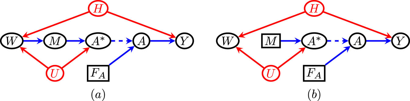
(a) The DT framework version of the napkin model. Only interventions on A are well-defined. (b) A graph representing the model where the variable M is “fixed” via the application of the truncated factorization.

Since q ( W , A ∗ , A , Y , U , H ∣ M , F A ) is Markov with respect to Figure 3(b), it also obeys independence restrictions given by the d-separation criterion in this graph. In particular, Y ⊥ ⊥ F A ∣ A , M , which implies q ( Y ∣ A = a , F A = a , M ) = q ( Y ∣ A = a , F A = ∅ , M ) , where

The reason for the equality q ( Y ∣ A = a , F A = a , M ) = p ( Y ∣ A = a , F A = a ) is somewhat subtle, but may be derived by comparing the Markov factorizations of q ( W , A ∗ , A , Y , U , H ∣ M , F A ) and p ( W , M , A ∗ , A , Y , U , H ∣ F A ) with respect to their appropriate (conditional) DAGs. Specifically, q ( Y ∣ A = a , F A = a , M ) and p ( Y ∣ A = a , F A = a ) are both functions of a fragment of the factorizations of those two distributions that remains invariant regardless of whether the fixing operation on M was performed.

Derivations of the above sort, which reason about distributions where only some variables may be intervened on, correspond more closely to how subject matter experts think about variables and their causal relationships in practice. However, obtaining such derivations in general problems seems to not be entirely obvious if interventions are restricted.

4 Conclusion

I want to thank Professor Dawid for writing such a stimulating paper. Professor Dawid views the DT framework as a harmonious influence in the “babel” of different voices advocating for different causal inference frameworks. My take is slightly different: I think the DT framework is a lovely corner in a garden where a thousand flowers bloom.

References

[1] Dawid AP. Influence diagrams for causal modelling and inference. Int Statist Rev. 2002;70:161–89. 10.1111/j.1751-5823.2002.tb00354.xSearch in Google Scholar
[2] Dawid AP. Counterfactuals, hypotheticals and potential responses: a philosophical examination of statistical causality. In: Russo F, Williamson J, editors. Causality and probability in the sciences, texts in philosophy. Vol. 5. London: College Publications; 2007. p. 503–32. Search in Google Scholar
[3] Dawid AP. Statistical causality from a decision-theoretic perspective. Annual Rev Statist Appl. 2015;2:273–303. 10.1146/annurev-statistics-010814-020105Search in Google Scholar
[4] Rubin DB. Causal inference and missing data (with discussion). Biometrika. 1976;63:581–92. 10.1093/biomet/63.3.581Search in Google Scholar
[5] Robins JM. A new approach to causal inference in mortality studies with sustained exposure periods – application to control of the healthy worker survivor effect. Math Model. 1986;7:1393–512. 10.1016/0270-0255(86)90088-6Search in Google Scholar
[6] Richardson TS, Robins JM. Single world intervention graphs (SWIGs): A unification of the counterfactual and graphical approaches to causality. 2013. Preprint: http://wwwcssswashingtonedu/Papers/wp128pdf. Search in Google Scholar
[7] Pearl J. Reasoning, and inference. 2nd ed. Cambridge, UK: Cambridge University Press; 2009. Search in Google Scholar
[8] Richardson TS, Evans RJ, Robins JM, Shpitser I. Nested Markov properties for acyclic directed mixed graphs. 2017. Working paper. Search in Google Scholar
[9] Shpitser I, Richardson TS, Robins JM. Multivariate counterfactual systems and causal graphical models. 2020. https://arxiv.org/abs/2008.06017. Search in Google Scholar
[10] Lauritzen SL, Richardson TS. Chain graph models and their causal interpretations (with discussion). J R Statist Soc B. 2002;64:321–61. 10.1111/1467-9868.00340Search in Google Scholar
[11] Sherman E, Shpitser I. Identification and estimation of causal effects from dependent data. In: Advances in neural information processing systems. Vol. 31. NY, United States: Curran Associates Inc.; 2018. Search in Google Scholar
[12] Sherman E, Shpitser I. General identification of dynamic treatment regimes under interference. In: Proceedings of the 21st International Conference on Artificial Intelligence and Statistics (AISTATS 2020). 2020. Search in Google Scholar
[13] Tchetgen Tchetgen EJ, Fulcher I, Shpitser I. Auto-G-computation of causal effects on a network. J Am Statist Assoc. 2020;116(534):833–44.10.1080/01621459.2020.1811098Search in Google Scholar PubMed PubMed Central
[14] Dawid AP. Beware of the DAG! In: Proceedings of Workshop on Causality: Objectives and Assessment at NIPS. vol. 6. 2010. p. 59–86. Search in Google Scholar
[15] Fulcher IR, Shpitser I, Marealle S, Tchetgen Tchetgen EJ. Robust inference on population indirect causal effects: the generalized front-door criterion. J R Statist Soc. B. 2019;82(1):199–214. 10.1111/rssb.12345Search in Google Scholar PubMed PubMed Central
[16] Didelez V. Causal concepts and graphical models. In: Handbook of Graphical Models. Boca Raton, FL: CRC Press; 2017. 10.1201/9780429463976-15Search in Google Scholar
[17] Malinsky D, Shpitser I, Richardson TS. A potential outcomes calculus for identifying conditional path-specific effects. In: Proceedings of the 22nd International Conference on Artificial Intelligence and Statistics. 2019. Search in Google Scholar
[18] Pearl J, MacKenzie D. The book of why: the new science of cause and effect. New York: Basic Books; 2018. Search in Google Scholar
[19] Verma TS, Pearl J. Equivalence and synthesis of causal models. Department of Computer Science. Los Angeles: University of California; 1990. p. R–150. Search in Google Scholar
[20] Forre P, Mooij JM. Causal calculus in the presence of cycles, latent confounders and selection bias. In: Proceedings of The 35th Uncertainty in Artificial Intelligence Conference. 2020. Search in Google Scholar
© 2022 Ilya Shpitser, published by De Gruyter
This work is licensed under the Creative Commons Attribution 4.0 International License.
Articles in the same Issue
- Editorial
- Causation and decision: On Dawid’s “Decision theoretic foundation of statistical causality”
- Research Articles
- Simple yet sharp sensitivity analysis for unmeasured confounding
- Decomposition of the total effect for two mediators: A natural mediated interaction effect framework
- Causal inference with imperfect instrumental variables
- A unifying causal framework for analyzing dataset shift-stable learning algorithms
- The variance of causal effect estimators for binary v-structures
- Treatment effect optimisation in dynamic environments
- Optimal weighting for estimating generalized average treatment effects
- A note on efficient minimum cost adjustment sets in causal graphical models
- Estimating marginal treatment effects under unobserved group heterogeneity
- Properties of restricted randomization with implications for experimental design
- Clarifying causal mediation analysis: Effect identification via three assumptions and five potential outcomes
- A generalized double robust Bayesian model averaging approach to causal effect estimation with application to the study of osteoporotic fractures
- Sensitivity analysis for causal effects with generalized linear models
- Individualized treatment rules under stochastic treatment cost constraints
- A Lasso approach to covariate selection and average treatment effect estimation for clustered RCTs using design-based methods
- Bias attenuation results for dichotomization of a continuous confounder
- Review Article
- Causal inference in AI education: A primer