Generalizing Experimental Findings

1 Transportability and selection bias

The long-standing problem of generalizing experimental findings from the trial sample to the population as a whole, also known as the problem of “sample selection-bias” [1, 2], has received renewed attention in the past decade, as more researchers come to recognize this bias as a major threat to the validity of experimental findings in both the health sciences [3] and social policy making [4]. Since participation in a randomized trial cannot be mandated, we cannot guarantee that the study population would be the same as the population of interest. For example, the study population may consist of volunteers, who respond to financial and medical incentives offered by pharmaceutical firms or experimental teams, so, the distribution of outcomes in the study may differ substantially from the distribution of outcomes under the policy of interest.

Another impediment to the validity of experimental finding is that the types of individuals in the target population may change over time [5]. For example, as more individuals become eligible for health insurance, the types of individuals seeking services would no longer match the type of individuals that were sampled for the study [3]. A similar change would occur as more individuals become aware of the efficacy of the treatment. The result is an inherent disparity between the target population and the population under study.

The problem of generalizing across disparate populations has received a formal treatment in Pearl and Bareinboim [6] where it was labeled “transportability,” and where necessary and sufficient conditions for valid generalization were established (see [7]). The problem of selection bias, though it has some unique features, can also be viewed as a nuance of the transportability problem, thus inheriting all the theoretical results established in Pearl and Bareinboim [6] that guarantee valid generalizations. I will describe the two problems side by side and then return to the distinction between the type of assumptions that are needed for enabling generalizations.

The transportability problem concerns two dissimilar populations, Π and Π∗, and requires us to estimate the average causal effect P∗(yx) (explicitly: P∗(yx)=ΔP∗(Y=y|do(X=x)) in the target population Π∗, based on experimental studies conducted on the source population Π. ^[1] Formally, we assume that all differences between Π and Π∗ can be attributed to a set of factors S that produce disparities between the two, so that P∗(yx)=P(yx|S=1). The information available to us consists of two parts; first, treatment effects estimated from experimental studies in Π and, second, observational information extracted from both Π and Π∗. The former can be written P(y|do(x),z), where Z is set of covariates measured in the experimental study, and the latters are written P∗(x,y,z)=P(x,y,z|S=1), and P(x,y,z) respectively. In addition to this information, we are also equipped with a qualitative causal model M, that encodes causal relationships in Π and Π∗, with the help of which we need to identify the query P∗(yx). Mathematically, identification amounts to transforming the query expression

into a form derivable from the available information ITR, where

The first two components of ITR represent, respectively, the experimental and observational findings in Π, while the third component represents observational findings in Π∗. Appendix 1 demonstrates how the query P∗(yx) can be derived from ITR using assumptions about the disparities between Π and Π∗ that are encoded in a graph.

The selection bias problem is slightly different. Here the aim is to estimate the average causal effect P(yx) in the Π population, while the experimental information available to us, ISB, comes from a preferentially selected sample, S=1, and is given by P(y|do(x),z,S=1). In addition, we also assume to have access to observational information P(x,y,z|S=1) and P(x,y,z); the first represents observations obtained from the selected sample, S=1, and the second represents observation taken on the population at large. Thus, the selection bias problem calls for transforming the query P(yx) to a form derivable from the information set:

In the Appendix section, we demonstrate how transportability problems and selection bias problems are solved using the transformations described above. At this point, however, it is important to note the syntactic differences between the information sets available in the two problems. ITR is characterized by the fact that S does not appear in the conditioning part of any do-expression, thus reflecting the fact that we do not have experimental information from the target population Π∗. ISB on the other hand is characterized by the fact that do-expressions are always conditioned on S, reflecting the fact that we have experimental information only on the selected sample, S=1.

The analysis reported in Pearl and Bareinboim [6] has resulted in an algorithmic criterion for deciding whether transportability is feasible and, when confirmed, the algorithm produces an estimand for the desired effects [7]. The algorithm is complete, in the sense that, when it fails, a consistent estimate of the target effect does not exist (unless one strengthens the assumptions encoded in M).

There are several lessons to be learned from this analysis when considering generalizing experimental findings.

1. The graphical criteria that authorize transportability are applicable to selection bias problems as well, provided that the graph structures for the two problems are identical. This means that whenever a selection bias problem is characterized by a graph for which transportability is feasible, recovery from selection bias is feasible by the same algorithm. (The Appendix demonstrates this correspondence.)

2. The assumptions needed for transportability are more involved than the ones usually invoked for ensuring non-confoundedness, also called “treatment assignment ignorability.” In graphical terms, these assumptions may require several d-separation tests on several sub-graphs. It is utterly unimaginable therefore that such assumptions could be managed by unaided human judgment, as is normally assumed in the potential outcomes literature [3, 9].

3. In general, problems associated with generalizing across populations cannot be handled by balancing disparities between distributions. A given disparity between P(x,y,z) and P∗(x,y,z) may demand different adjustments, depending on the location of S in the causal structure. A simple example of this phenomenon is demonstrated in Figure 3(b) of [6] where a disparity in the average reading ability of two cities requires two different treatments, depending on what causes the disparity. If the disparity emanates from age differences, adjustment is necessary, because age is likely to affect the potential outcomes. If, on the other hand the disparity emanates from differences in educational programs, no adjustment is needed, since education, in itself, does not modify response to treatment. Such distinctions, which may become quite intricate in large systems, are managed automatically in the graph-based representation.

4. In many instances, generalizations can only be achieved by conditioning on post-treatment variables, an operation that is generally frowned upon in the potential outcomes [10, pp. 73–74, 11, 12]; but has become extremely useful in graphical analysis. The difference between the conditioning operators used in these two frameworks is reflected in the difference between the counterfactual expression P(Yx=y|z) and the do-expression P(Y=y|do(X=x),z) [13]. The latter expression defines information that is estimable directly from experimental studies, whereas the former invokes retrospective counterfactuals that may or may not be estimable empirically.

2 Ignorability versus admissibility in the pursuit of generalizations

A key assumption in almost all conventional analyses of generalization (from sample-to-population) is S-ignorability, written

where Yx is the potential outcome predicated on the intervention X=x, S is a selection indicator (with S=1 standing for selection into the sample) and Z a set of observed covariates. This assumption, commonly written as a difference Y1−Y0⊥⊥S|Z, appears in Hotz et al. [5]; Cole and Stuart [14]; Tipton et al. [15]; Hartman et al. [9], and possibly other researchers confined to potential outcomes analysis. This assumption states that in every stratum Z=z of the set Z, the potential outcome Yx is independent of the factors S that may produce cross-population differences.

Given this assumption, the problem of generalizing across populations has a trivial solution, which reads: If we succeed in finding a set Z of pre-treatment covariates such that cross-population differences disappear in every stratum Z=z, then the problem can be solved by averaging over those strata. ^[2]

Specifically, if P(yx|S=1,Z=z) is the z-specific probability distribution of Yx in the sample, then the distribution of Yx in the population at large is given by the post-stratification formula

which is often referred to as re-calibration or re-weighting. Here, P(z) is the probability of Z=z in the target population (where S=0). Equation (5) follows from S-ignorability by conditioning on z and, adding S=1 to the conditioning set – a one-line proof. The proof fails however when no covariate set Z exists that satisfies S-ignorability, in which case the post-stratification formula will be invalid. Moreover, even when S-ignorability holds, eq. (5) would only be applicable if the factor P(yx|S=1,z) is estimable in the experimental study and this will generally not be the case when Z contains post-treatment variables (see [13], Figure 1).

Symmetrically, when we consider transportability problems, our query is P∗(yx)=P(y|do(x),S=1) (see eq. (1)), and S-ignorability would permit us to remove the S=1 condition and obtain the post-stratification formula

Similar to eq. (5), this formula takes a weighted average of the z-specific potential outcome Yx over all levels of Z. Here, in syntactic contrast, the average is weighed by P(z|S=1) which is, again, the distribution of Z in the target population (where S=1). As in the case of selection bias, eq. (6) is only useful when S-ignorability holds and when P(yx|z) is estimable from the experimental data. Unfortunately, when Z contains post-treatment variables, the former condition will be harder to meet; we shall see that S-ignorability is rarely satisfied in transportability problems by any set Z containing post-treatment variables.

In graphical analysis, on the other hand, the problem of generalization has been studied using another assumption, labeled S-admissibility [7], which is defined by:

or, using counter factual notation,

It states that in every treatment regime X=x, the observed outcome Y is conditionally independent of the selection mechanism S, given Z, all evaluated at that same treatment regime.

Clearly, S-admissibility coincides with S-ignorability for pretreatment S and Z; the two notions differ however for treatment-dependent selection and covariates. To witness, consider the model of Figure 1(a), and let X stand for education, Z for skill, S for training, and Y for salary.

Figure 1:

(a) A transportability model in which a post-treatment variable Z is S-admissible but not S-ignorable; (b) A selection-bias model in which Z is both S-admissible and S-ignorable. Note that S is a root node in (a) and a sink node in (b), where it is a proxy of Z. In both models, the post-stratification formula (5) is not estimable non-parametrically.

S-admissibility eq. (4) looks at those people who were assigned x years of education who subsequently achieved skill level z, and asks whether their salary Y would depend on their training S. The graph states that skill alone determines salary, not how it was acquired, therefore P(y|do(x),z))=P(y|do(x),z,s)=P(y|z) namely, training and education have no effect on salary, once we know z, as shown in the graph.

In contrast, S-ignorability Yx⊥⊥S|Z asks for the role that training plays in the salary of those individuals who are currently at skill Z=z, had they received x years of schooling. Surely, unless x is pathologically low, the skill levels attained by these individuals would depend on the amount of training (S) they receive, and so would their salary Y. We thus conclude that Yx is not independent of S given Z, namely, S-ignorability does not hold. The condition Z=z merely selects a subpopulation for consideration but, unless individuals in this subpopulation possess some abnormal qualities, they should exhibit the natural dependence of salary on training. ^[3]

The Appendix section shows that unbiased generalization across studies is indeed feasible in scenarios like Figure 1(a), despite the fact that Z is not S-ignorable. This is facilitated by the fact that Z is S-admissible, since Z separates Y from S in the graph, and leads to the following estimand for the target effect:

Note that this estimand invokes nonconventional average of the z-specific effect, weighted by the conditional probability P(z|x) at the target population.

A similar situation occurs in sample-selection problems such as the one depicted in Figure 1(b), where generalization from samples to populations through the post-stratification formula (5) requires S-ignorability. Here, the post-stratification formula (5) is valid because Z is S-ignorable (Z separates S from Yx in the graph), yet the formula is useles, because the z-specific causal effect P(yx|S=1,z) is not estimable from the experimental study.

Remarkably, the target distribution P(yx) can be estimated using a modified formula:

which follows from the fact that Z is S-admissible. The derivation is presented in Scenario 3 of the Appendix and demonstrates that, regardless of whether Z satisfies S-ignorability or S-admissibility, experimental findings are not generalizable by standard procedures of post-stratification. Rather, modified procedures need be applied, dictated by the graph structure.

One of the reasons that S-admissibility has received greater attention in the graph-based literature is that it has a very simple graphical representation: Z and X should separate Y from S in a mutilated graph, from which all arrows entering X have been removed. Such a graph depicts conditional independencies among observed variables in the population under experimental conditions, i.e., where X is randomized.

S-ignorability requires a more elaborate graphical interpretation; it can be verified from either twin networks [16, pp. 213–4] or from counterfactually augmented graphs [16, p. 341]. Using either representation, it is easy to see that S-ignorability is rarely satisfied in problems in which Z is a post-treatment variable. This is because, whenever S is an ancestor of Z, or a proxy of such ancestor, Z cannot separate Yx from S.

As noted in Keiding [17] the re-calibration formula (5) goes back to eighteenth century demographers [18, 19] facing the task of predicting overall mortality (across populations) from age-specific data. Their reasoning was probably as follows: If the source and target populations differ in distribution by a set of attributes Z, then to correct for these differences we need to weight samples by a factor that would restore similarity to the two distributions. Some researchers view eq. (5) as a version of Horvitz and Thompson [20] post-stratification method of estimating the mean of a super-population from un-representative stratified samples. The essential difference between survey sampling calibration and the calibration required in eq. (5) is that the calibrating covariates Z are not just any set by which the distributions differ; they must satisfy the S-ignorability (or admissibility) condition, which is a causal, not a statistical condition and is not discernible therefore from distributions over observed variables. In other words, the re-calibration formula should depend on disparities between the causal models of the two populations, not merely on distributional disparities; we discussed this point in Section 1 (item 3) and it is also demonstrated in the Appendix (Figure 2(a)). While S-ignorability and S-admissibility are both sufficient for re-calibrating pre-treatment covariates Z, S-admissibility goes further and discovers generalizations that leverage both pre-treatment and post-treatment variables. The three examples discussed in the Appendix demonstrate this point.

Figure 2:

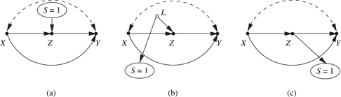
(a) Generalizable transportability problem in which Z is S-admissible but S-ignorability does not hold. (b) Generalizable selection-bias problem in which Z is S-admissible but S-ignorability does not hold. (c) Generalizable selection-bias problem in which S-admissibility and S-ignorability both hold, yet post-stratification (eq. (5)) fails to estimate the target treatment effect P(yx).

3 Conclusions

1. Many opportunities for generalization are opened up through the use of post-treatment variables. These opportunities remain inaccessible to ignorability-based analysis, partly because S-ignorability does not always hold for such variables but, mainly, because ignorability analysis requires information in the form of z-specific counterfactuals, which is often not estimable from experimental studies.

2. Most of these opportunities have been chartered through the completeness results for transportability [1], others can be revealed by simple derivations in do-calculus as shown in the Appendix.

3. There is still the issue of assisting researchers in judging whether S-ignorability (or S-admissibility) is plausible in any given application. Graphs excel in this dimension because they match the format in which people store scientific knowledge. Researchers who insist on discerning S-ignorability by appealing to human intuition do so at the peril of missing opportunities for generalization, or producing biased effect estimates. Readers can appreciate the magnitude of these perils by examining the simple examples presented in Figure 2 of the Appendix; discerning S-ignorability in any one of the three scenarios is a formidable judgmental task if unaided by graphs.